Meetup 5: Data Transformation

George I. Hagstrom

2025-09-22

Week Summary

• Reading: Chapters 12, 13, 17 of R4DS
• Lab 4 on Data Transformations Due Sunday at Midnight

Common Questions: What Graph?

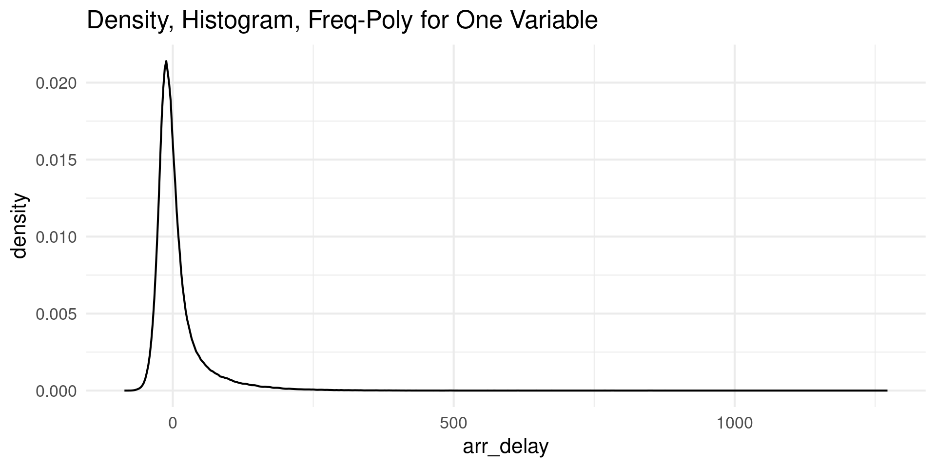
• One Continuous variable
• Density plot, histogram, frequency polygon (geom_density, geom_histogram, geom_freqpoly)

Common Questions: What Graph?

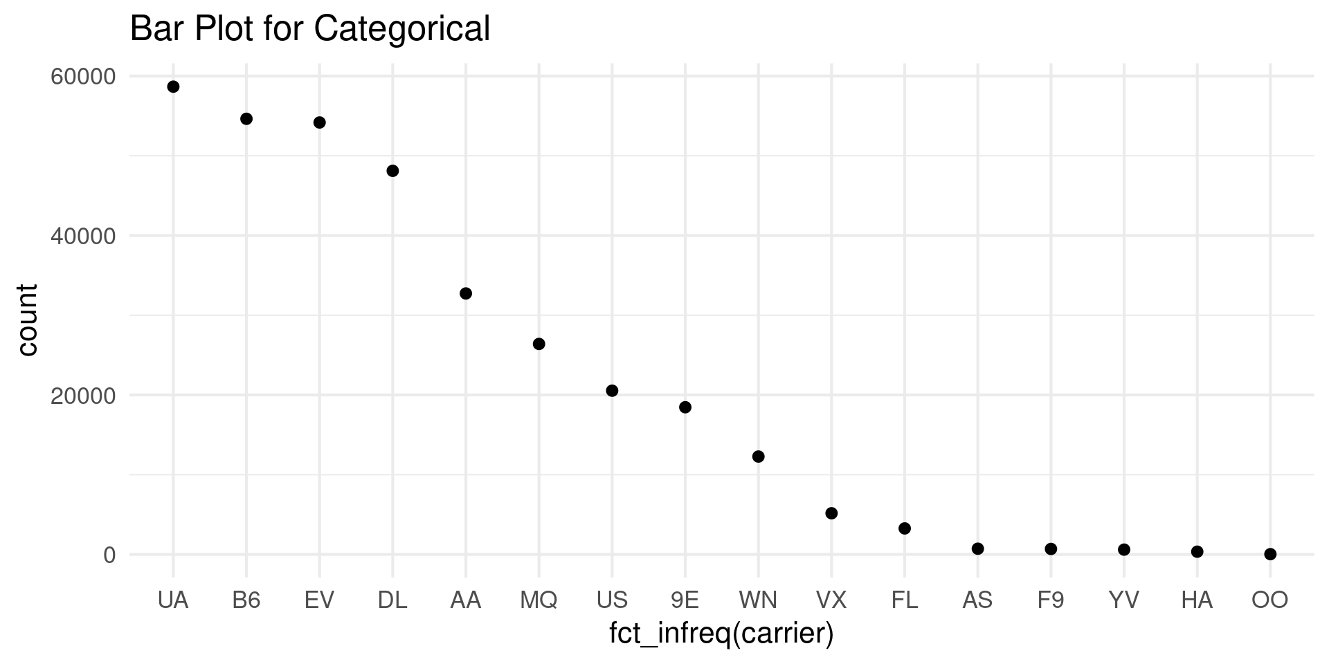
• One Categorical variable
• Bar Plot, dot plot (geom_bar, geom_point with stat="count")

Common Questions: What Plot?

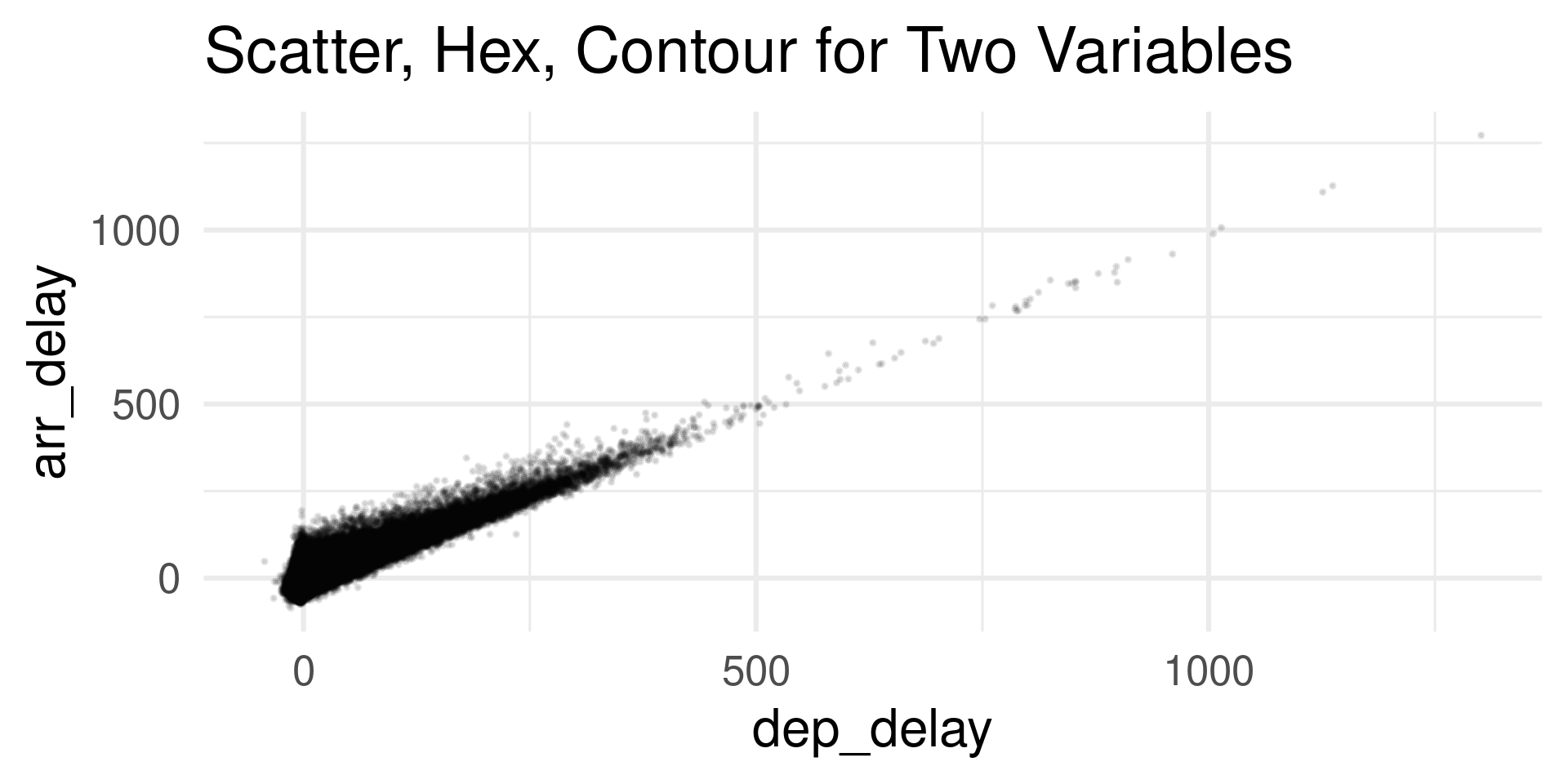
• Two Numerical variables
• geom_point, geom_hex, geom_contour

Common Questions: What Plot?

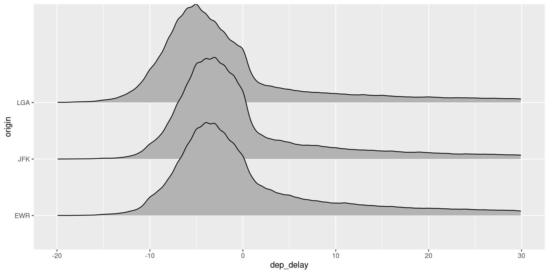
• Numerical and Categorical
• geom_density_ridges, geom_boplot, geom_violin
• Use other aesthetics (fill), use facets

Common Questions: What Plot?

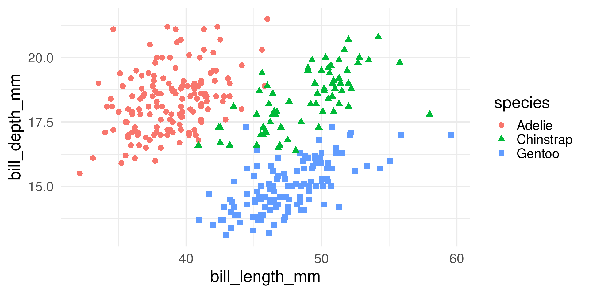
• Two numerical and one categorical
• Faceted Scatterplot or other aesthetics

Common Questions: What Plot?

• One Numerical and multiple categorical
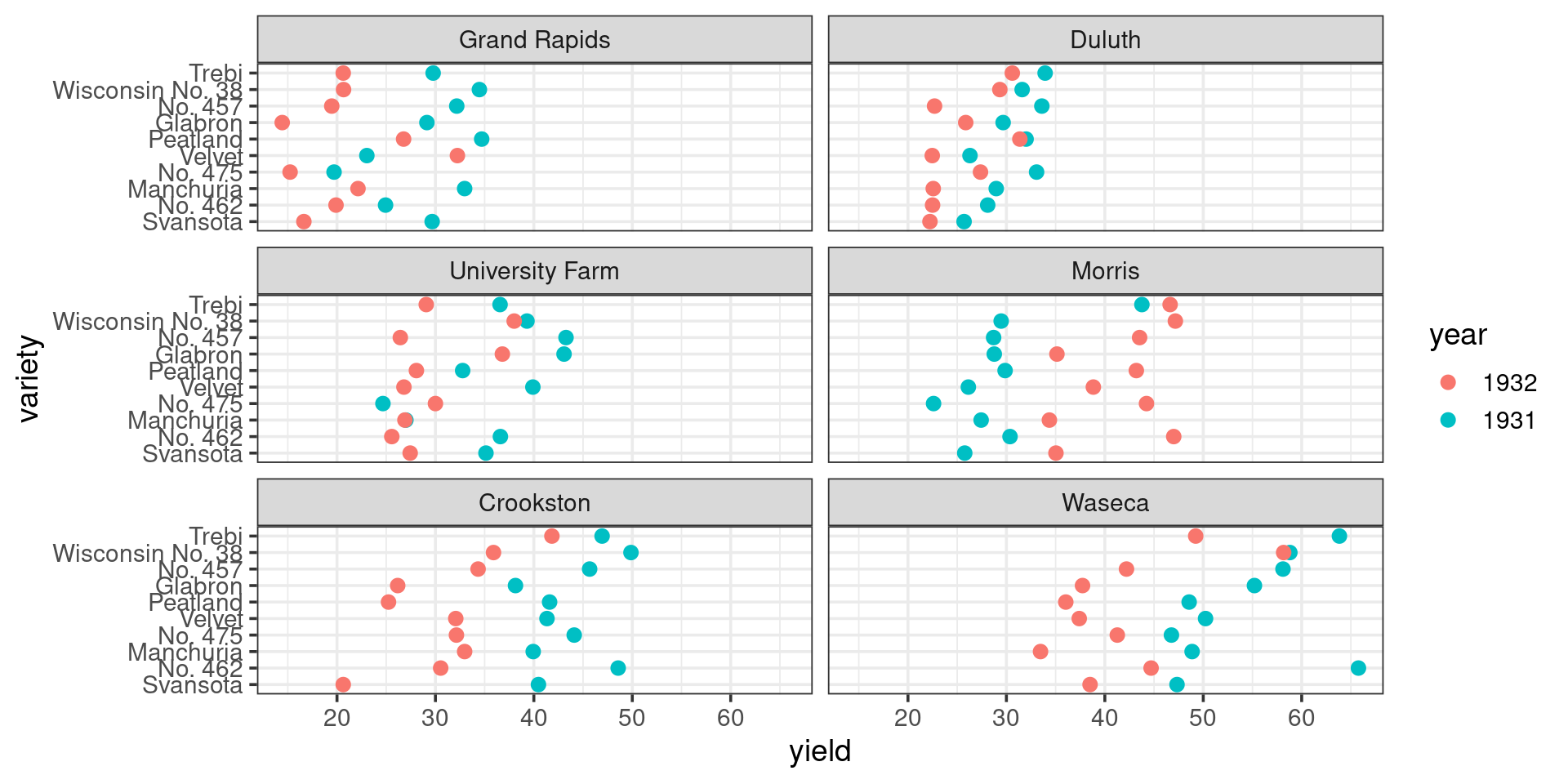
• Multiway dot plot

Common Questions: What Plot?

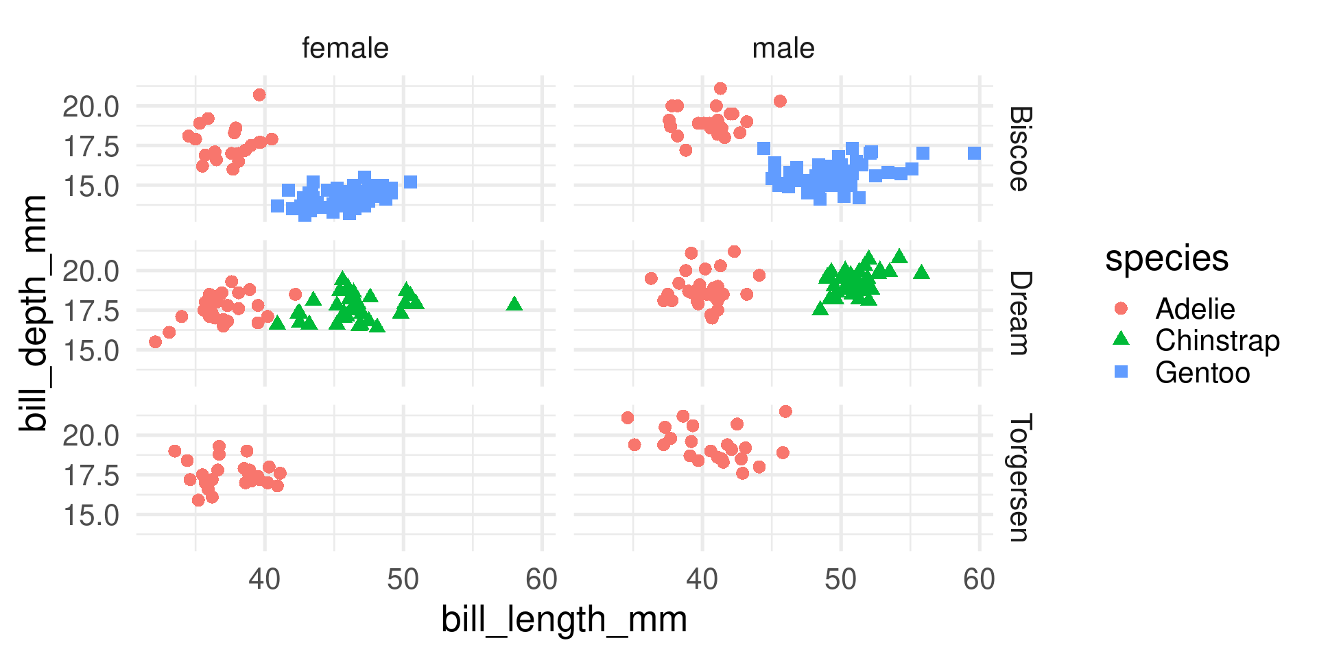
• You can keep going in this direction, but gets harder to understand
• Multiple categorical and numerical, can use facets, aesthetics, do a scatterplot etc

Data Transformation

• Process of creating new variables from current data
• Needed to prepare data for your analyses and questions
• Data transformations can lead to dramatically improved insight at little cost
• Types: Numbers, logical variables, dates, later strings and factors.

Case Study: Brain and Body Size

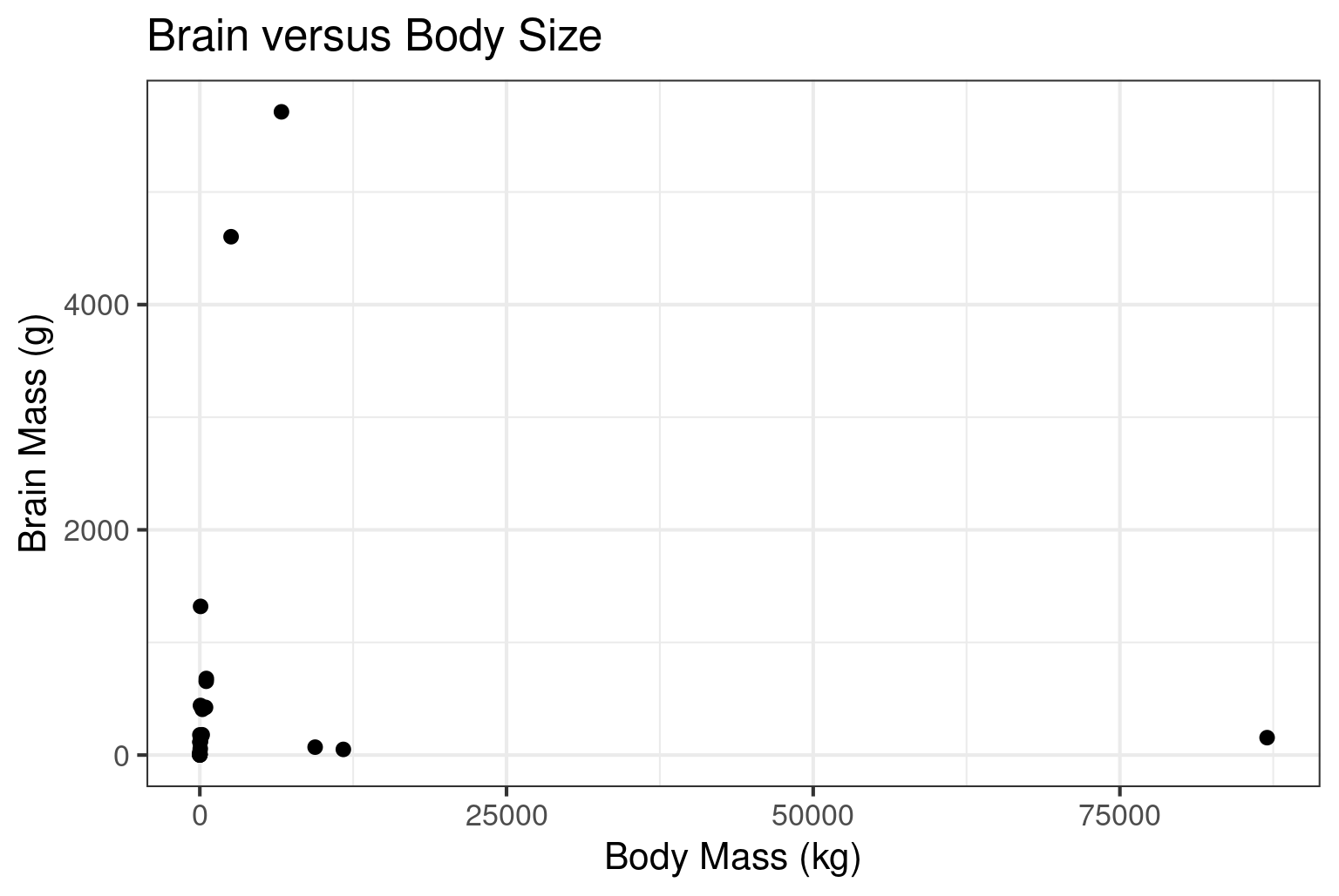
No Correlation?

• Compute the Pearson correlation between brain mass and body mass:

cor(Animals$body,Animals$brain)

[1] -0.005341163

• We expect a strong relationship between brain mass and body mass
• Very difficult to believe that there is no relationship between brain mass and body mass.

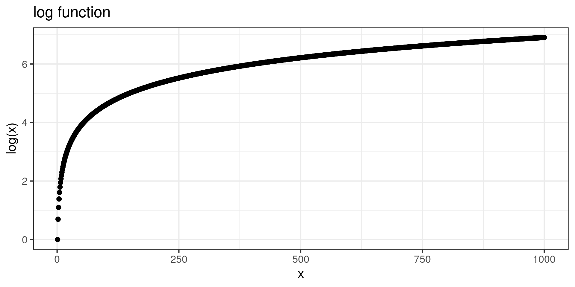
Log Transformation

• Brain and Body size:
  • Positive variables
  • Range over orders of magnitude
  • Result from multiplicative growth processes
• Suggests we try logarithms

xkcd

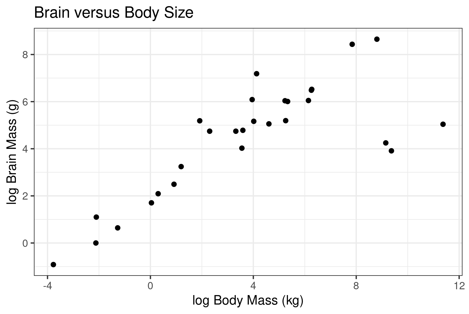
Log Transformation: Different Story

Animals |> 
  summarize(Correlation = cor(log(body),log(brain)) ) |> print()

  Correlation
1   0.7794935

Boolean/Logical Operations

• Logical Types: TRUE and FALSE
• NOT: !TRUE = FALSE, !FALSE=TRUE
• AND: only TRUE & TRUE = TRUE rest FALSE
• OR: only FALSE | FALSE = FALSE rest TRUE

Comparison statements don’t work like in English:

4 > 5 | 6 # Wrong

[1] TRUE

(4 > 5) | (4 > 6) # Right

[1] FALSE

Boolean Variables for Comparison

library(kableExtra)
nycflights13::flights |> select(year,month,day,arr_delay,carrier,origin,dest) |>  head(10) |> kable()

year	month	day	arr_delay	carrier	origin	dest
2013	1	1	11	UA	EWR	IAH
2013	1	1	20	UA	LGA	IAH
2013	1	1	33	AA	JFK	MIA
2013	1	1	-18	B6	JFK	BQN
2013	1	1	-25	DL	LGA	ATL
2013	1	1	12	UA	EWR	ORD
2013	1	1	19	B6	EWR	FLL
2013	1	1	-14	EV	LGA	IAD
2013	1	1	-8	B6	JFK	MCO
2013	1	1	8	AA	LGA	ORD

Compare DL, UA, AA to others

• Create variable that is TRUE when airline is in the group
• FALSE otherwise

flights = nycflights13::flights |> 
  mutate(IS_CARRIER_DL_UA_AA = carrier %in% c("DL","UA","AA"))
flights |> 
  group_by(IS_CARRIER_DL_UA_AA) |> 
  summarise(fraction_delayed = sum(arr_delay>30,na.rm=TRUE)/
              sum(is.finite(arr_delay),na.rm=TRUE)) |> 
  print()

# A tibble: 2 × 2
  IS_CARRIER_DL_UA_AA fraction_delayed
  <lgl>                          <dbl>
1 FALSE                          0.180
2 TRUE                           0.125

Logical Subsetting

• Powerful way of manipulating Data Frames
• if_else and case_when: vector output

diamonds |> 
  mutate( cut = if_else(
      cut == "Very Good", "Very_Good", cut)
    )

Logical Subsetting using Base

• Can use [] for other data types

diabetes = read_csv("../../assignments/labs/labData/diabetes.csv")
diabetes

# A tibble: 768 × 9
   Pregnancies Glucose BloodPressure SkinThickness Insulin   BMI
         <dbl>   <dbl>         <dbl>         <dbl>   <dbl> <dbl>
 1           6     148            72            35       0  33.6
 2           1      85            66            29       0  26.6
 3           8     183            64             0       0  23.3
 4           1      89            66            23      94  28.1
 5           0     137            40            35     168  43.1
 6           5     116            74             0       0  25.6
 7           3      78            50            32      88  31  
 8          10     115             0             0       0  35.3
 9           2     197            70            45     543  30.5
10           8     125            96             0       0   0  
# ℹ 758 more rows
# ℹ 3 more variables: DiabetesPedigreeFunction <dbl>, Age <dbl>, Outcome <dbl>

Logical Subsetting using Base

• Can use [] for other data types

diabetes[2:6][diabetes[2:6]==0] = NA
diabetes

# A tibble: 768 × 9
   Pregnancies Glucose BloodPressure SkinThickness Insulin   BMI
         <dbl>   <dbl>         <dbl>         <dbl>   <dbl> <dbl>
 1           6     148            72            35      NA  33.6
 2           1      85            66            29      NA  26.6
 3           8     183            64            NA      NA  23.3
 4           1      89            66            23      94  28.1
 5           0     137            40            35     168  43.1
 6           5     116            74            NA      NA  25.6
 7           3      78            50            32      88  31  
 8          10     115            NA            NA      NA  35.3
 9           2     197            70            45     543  30.5
10           8     125            96            NA      NA  NA  
# ℹ 758 more rows
# ℹ 3 more variables: DiabetesPedigreeFunction <dbl>, Age <dbl>, Outcome <dbl>

Numerical Transformations

• Can implement any mathematical formula you can imagine
• Construct quantity of interest:
  • Domain expertise
• As part of EDA
  • Make a complicated relationship look simpler or even linear
• To boost other tools
  • Some algorithms run better with standardized data

Defining Functions

• For complicated data transformations, define a function

my_transformation = function(var1,var2,kfact = 1){
  
  mean_var1 = mean(var1)
  sd_var1 = sd(var1)
  mean_var2 = mean(var2)
  sd_var2 = sd(var2)
  return(exp(-kfact*abs((var1-mean_var1)*(var2-mean_var2))/(sd_var1*sd_var2)))
  
}

• Functions make code easier to read
• Write function when code reused 3 times

Recycling Rules for Aggregates

• R “boosts” numbers/vectors so that calculations work
• Behavior is very different from other languages:

c(5,2,3,10)/c(1,9,1)

[1]  5.0000000  0.2222222  3.0000000 10.0000000

• Shorter vector/number is repeated to match the length of longer one
• Can be very unintuitive for when the vectors have lengths different from 1

Recycling Fails:

• Source of silent bugs

flights |> 
  filter(month == c(1, 2)) |> select(year, month, flight) |> head(5)

# A tibble: 5 × 3
   year month flight
  <int> <int>  <int>
1  2013     1   1545
2  2013     1   1141
3  2013     1    461
4  2013     1    507
5  2013     1     79

flights |> 
  filter(month %in% c(1, 2)) |> select(year, month, flight) |> head(5)

# A tibble: 5 × 3
   year month flight
  <int> <int>  <int>
1  2013     1   1545
2  2013     1   1714
3  2013     1   1141
4  2013     1    725
5  2013     1    461

logarithms

• \(\log(e^x) = x\)
• \(\log(x_1 \cdot x_2 \cdot \dots \cdot x_n) = \log(x_1) + \log(x_2) + \dots + \log(x_n)\)
• \(\log_{10}\) counts the digits of a number

\(\log\) in data science and stats

• Starting point when:
  • Positive variables
  • Multiplicative growth
  • Wide Range
• Avoiding overflow/underflow in probability models
  • In maximum likelihood focus on log likelihood
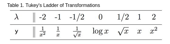
• Special case of Tukey’s Ladder:

Two Approaches to Transformations:

1. Domain Focused:

• Construct quantities of interest
• Transformation always inspired by knowledge of domain
• Power transformation to scale physical values

2. Stats Focused:

• Transform with goal to make data more Normal, relations more linear
• Exemplified by Box-Cox Transformation

Window Functions: Values

• Perform transformations on “nearby” rows:
• lead Next value(s)
• lag Previous value(s)

c(1,2,3,4,5,6,7,8,9,10) |> lead() 

 [1]  2  3  4  5  6  7  8  9 10 NA

c(1,2,3,4,5,6,7,8,9,10) |> lead(n=3) 

 [1]  4  5  6  7  8  9 10 NA NA NA

c(1,2,3,4,5,6,7,8,9,10) |> lag() 

 [1] NA  1  2  3  4  5  6  7  8  9

c(1,2,3,4,5,6,7,8,9,10) |> lag(n=3) 

 [1] NA NA NA  1  2  3  4  5  6  7

• first() and last()

Window Functions: Ranks

• Perform transformations on “nearby” rows:
• percent_rank()
• rank()
• ntile()

c(1,2,3,4,5,6,7,8,9,10) |> percent_rank() 

 [1] 0.0000000 0.1111111 0.2222222 0.3333333 0.4444444 0.5555556 0.6666667
 [8] 0.7777778 0.8888889 1.0000000

c(1,2,3,4,5,6,7,8,9,10) |> rank() 

 [1]  1  2  3  4  5  6  7  8  9 10

c(1,2,3,4,5,6,7,8,9,10) |> ntile(4) 

 [1] 1 1 1 2 2 2 3 3 4 4

Cumulative and Rolling Aggregates

• cumsum, cummean
• Rolling window (several libraries including RcppRoll, TTR, slider)

library(TTR)
library(cranlogs)
pkgs = c(
    "tidyr", "lubridate", "dplyr", 
    "ggplot2", "purrr", 
    "stringr", "knitr"
    )

tidyverse_downloads = cran_downloads(
    packages = pkgs, 
    from     = "2024-01-01", 
    to       = "2024-08-31") %>%
    tibble::as_tibble() %>%
    group_by(package)

Cumulative and Rolling Aggregates

• cumsum, cummean
• Rolling window (several libraries including RcppRoll, TTR, slider)

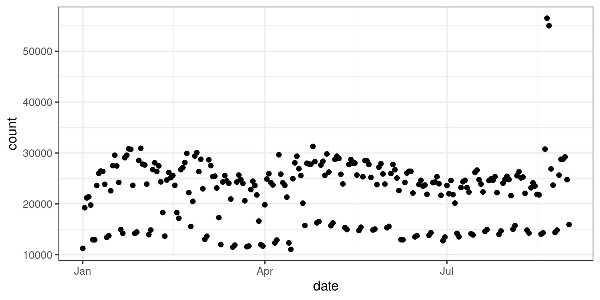
tidyverse_downloads |> filter(package == "lubridate") |> 
  ggplot(aes(x=date,y=count)) + geom_point()+
  theme_bw(base_size = 16)

Cumulative and Rolling Aggregates

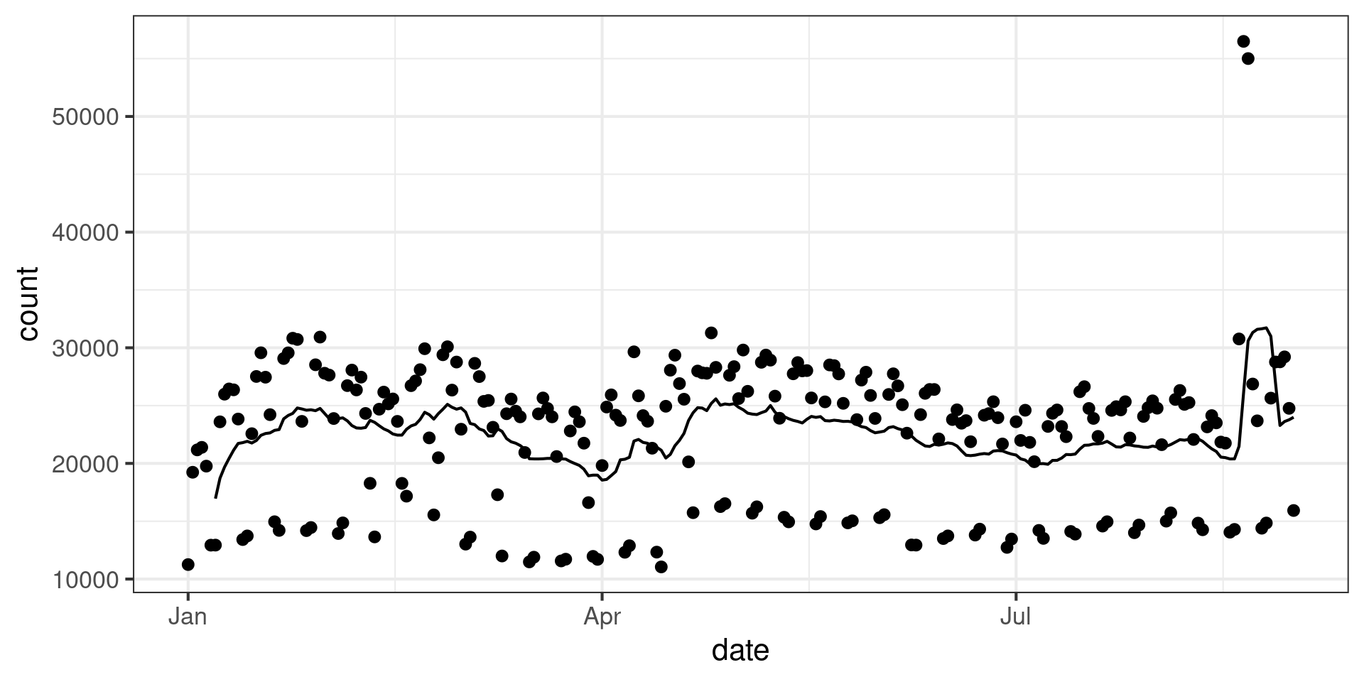
• Rolling window TTR:

tidyverse_downloads |> filter(package == "lubridate") |> 
  ggplot(aes(x=date,y=count)) + geom_point()+
  theme_bw(base_size = 16)

Cumulative and Rolling Aggregates

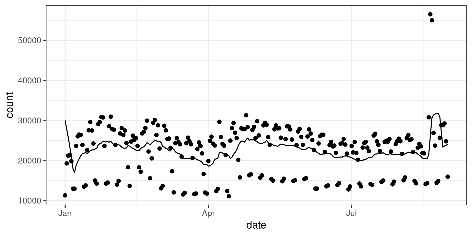
tidyverse_downloads |> filter(package == "lubridate") |> 
  mutate(rolling_count = runMean(count,n=7)) |> 
  ggplot(aes(x=date,y=count)) + geom_point() + geom_line(aes(y=rolling_count)) +
  theme_bw(base_size = 16)

Caution About Group Boundaries

tidyverse_downloads |>  ungroup() |> 
  mutate(rolling_count = runMean(count,n=7)) |> 
  filter(package == "lubridate") |> 
  ggplot(aes(x=date,y=count)) + 
  geom_point() + 
  geom_line(aes(y=rolling_count)) +
  theme_bw(base_size = 16)

Data Science in Context Presentation

Rank

• rank transforms data from values to numerical rank:

randVec = rnorm(10)
print(randVec)

 [1]  2.3018724  0.4560994  0.8971370  1.2285259 -0.5153130 -0.4754930
 [7] -1.0822176  1.7008024 -0.1618288  0.2311937

print(randVec |> rank())

 [1] 10  6  7  8  2  3  1  9  4  5

• Rank preserved by all monotone transformations

Rank and Correlation Trick

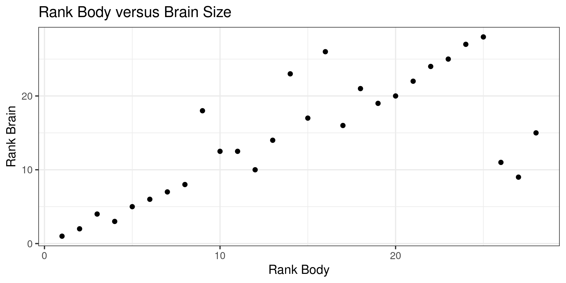
• Spearman Correlation is correlation between ranks of two variables

Animals  |> 
           summarise(
  rank_corr = cor(body,brain,method='spearman'),
  corr = cor(body,brain)
)

  rank_corr         corr
1 0.7162994 -0.005341163

• Correlation Trick: Look for Nonlinear Transformations when Rank-Correlation is much higher than Pearson Correlation

Rank Correlation Graphical Version

What didn’t we cover?

• logit, probit, ReLU: Data transformations that go between a finite interval and the real line
• Enormous number of different ranking functions available in R
• Linear Algebra Based Methods, PCA, dimensionality reduction
• Tools from the sciences: Fourier, Wavelets, etc

Meetup Reflection/One Minute Paper

Please fill out the following google form after the meeting or watching the video:

Click Here