DATA 608 Meetup 11: Clustering

George I. Hagstrom

Week Summary

Data Story 6 is available, due Sunday November 22
Last Data Story will be on Shiny Apps
Talking about clustering today

Clustering and Dim. Reduction

We can gain insight when we notice data points cluster together

Alcohol	Malic	Ash	Alcalinity	Magnesium	Phenols	Flavanoids	Nonflavanoids	Proanthocyanins	Color	Hue	Dilution	Proline
14.23	1.71	2.43	15.6	127	2.80	3.06	0.28	2.29	5.64	1.04	3.92	1065
13.20	1.78	2.14	11.2	100	2.65	2.76	0.26	1.28	4.38	1.05	3.40	1050
13.16	2.36	2.67	18.6	101	2.80	3.24	0.30	2.81	5.68	1.03	3.17	1185
14.37	1.95	2.50	16.8	113	3.85	3.49	0.24	2.18	7.80	0.86	3.45	1480
13.24	2.59	2.87	21.0	118	2.80	2.69	0.39	1.82	4.32	1.04	2.93	735
14.20	1.76	2.45	15.2	112	3.27	3.39	0.34	1.97	6.75	1.05	2.85	1450
14.39	1.87	2.45	14.6	96	2.50	2.52	0.30	1.98	5.25	1.02	3.58	1290
14.06	2.15	2.61	17.6	121	2.60	2.51	0.31	1.25	5.05	1.06	3.58	1295
14.83	1.64	2.17	14.0	97	2.80	2.98	0.29	1.98	5.20	1.08	2.85	1045
13.86	1.35	2.27	16.0	98	2.98	3.15	0.22	1.85	7.22	1.01	3.55	1045

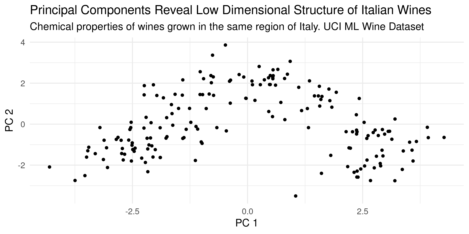
Clustering and Dim. Reduction

Color by the grape type

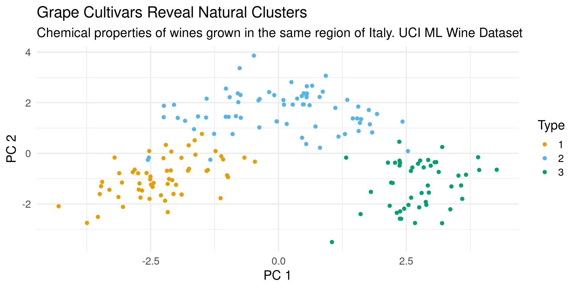
Automatic Clustering

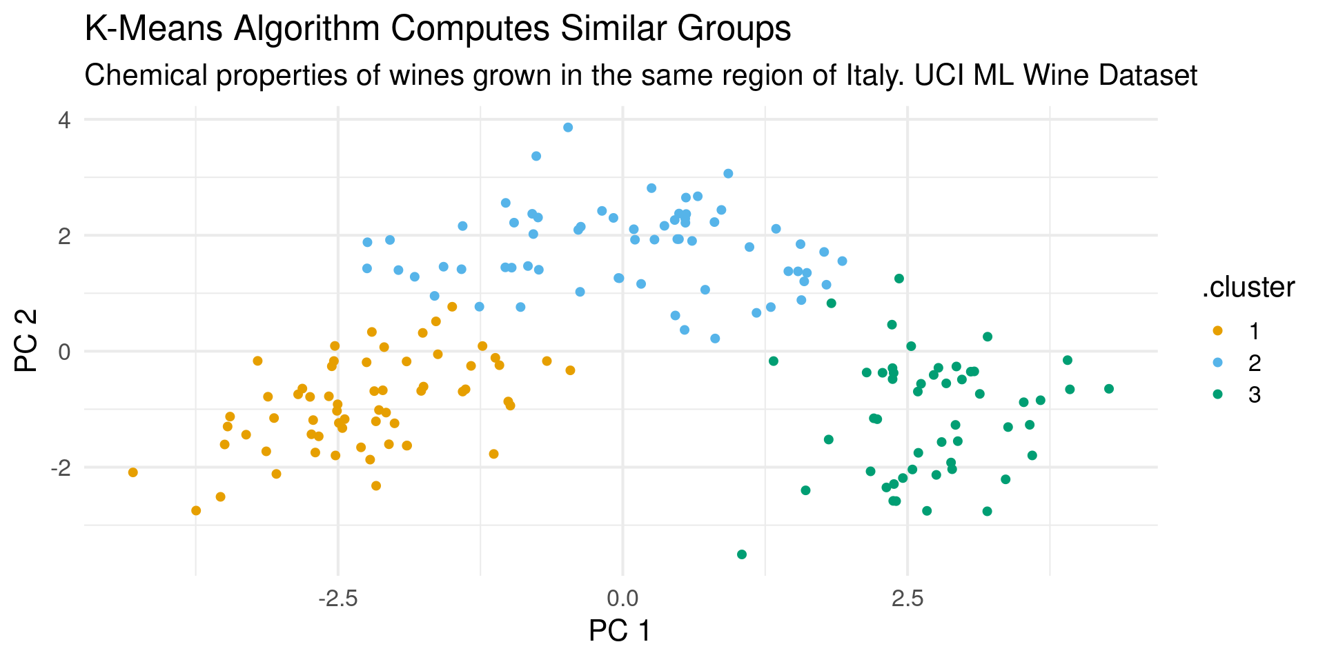
k-means method

Most common clustering method
Needs two things:
- Measure of distance between points
- Number of Clusters to find
Each cluster characterized by a center
Points clustered to closest center

k-means method

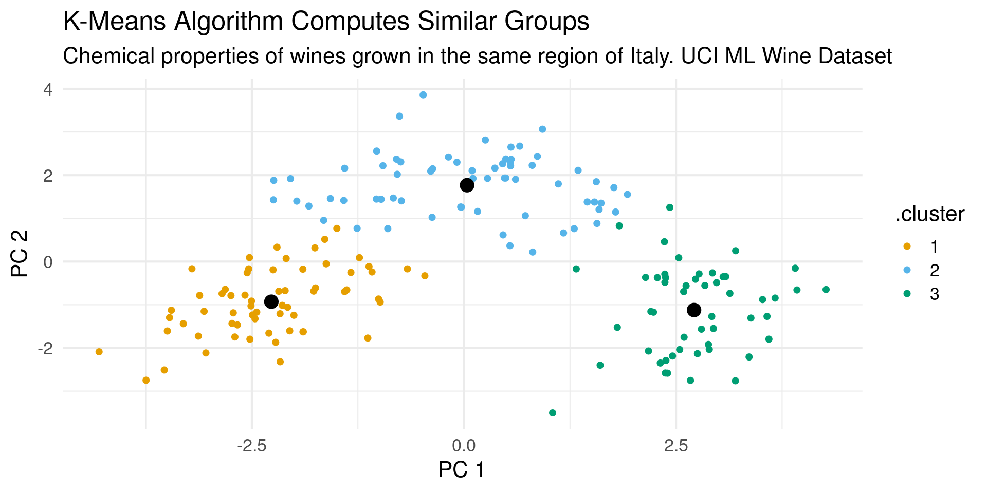
Implementing k-means in R

kmeans in stats package

wine_clusters = pca_fit|> 
    augment(wine_df) |> select(-Type) |> 
  select(.fittedPC1:.fittedPC13) |> 
  kmeans(centers=3,nstart = 10) 

wine_clusters

K-means clustering with 3 clusters of sizes 65, 62, 51

Cluster means:
   .fittedPC1 .fittedPC2   .fittedPC3  .fittedPC4  .fittedPC5  .fittedPC6
1  0.03685265  1.7672542  0.185615130  0.08001400 -0.07067870  0.12944063
2 -2.26979079 -0.9294322  0.001523733 -0.13511700  0.13453261 -0.21766922
3  2.71238444 -1.1224849 -0.238420685  0.06228125 -0.07346875  0.09964414
    .fittedPC7   .fittedPC8  .fittedPC9 .fittedPC10  .fittedPC11  .fittedPC12
1 -0.002320739 -0.017964647 -0.03216049  0.02293882  0.013900922  0.004371673
2  0.051963343  0.024894027  0.05014407 -0.07446923 -0.021230820 -0.007417378
3 -0.060213318 -0.007367207 -0.01997059  0.06129547  0.008093155  0.003445464
   .fittedPC13
1  0.008595707
2 -0.050476861
3  0.050408713

Clustering vector:
  [1] 2 2 2 2 2 2 2 2 2 2 2 2 2 2 2 2 2 2 2 2 2 2 2 2 2 2 2 2 2 2 2 2 2 2 2 2 2
 [38] 2 2 2 2 2 2 2 2 2 2 2 2 2 2 2 2 2 2 2 2 2 2 1 1 3 1 1 1 1 1 1 1 1 1 1 1 2
 [75] 1 1 1 1 1 1 1 1 1 3 1 1 1 1 1 1 1 1 1 1 1 2 1 1 1 1 1 1 1 1 1 1 1 1 1 1 1
[112] 1 1 1 1 1 1 1 3 1 1 2 1 1 1 1 1 1 1 1 3 3 3 3 3 3 3 3 3 3 3 3 3 3 3 3 3 3
[149] 3 3 3 3 3 3 3 3 3 3 3 3 3 3 3 3 3 3 3 3 3 3 3 3 3 3 3 3 3 3

Within cluster sum of squares by cluster:
[1] 558.6971 385.6983 326.3537
 (between_SS / total_SS =  44.8 %)

Available components:

[1] "cluster"      "centers"      "totss"        "withinss"     "tot.withinss"
[6] "betweenss"    "size"         "iter"         "ifault"

Key arguments

centers species the number of clusters to find
nstart is number of times to initialize algorithm
algorithm several choices the default choice is usually very robust
iter.max is the number of iterations to try

Key Outputs

Clustering Vector: Identifies each point by cluster. Is attached to original data frame by augmnet

wine_clusters$cluster

  [1] 2 2 2 2 2 2 2 2 2 2 2 2 2 2 2 2 2 2 2 2 2 2 2 2 2 2 2 2 2 2 2 2 2 2 2 2 2
 [38] 2 2 2 2 2 2 2 2 2 2 2 2 2 2 2 2 2 2 2 2 2 2 1 1 3 1 1 1 1 1 1 1 1 1 1 1 2
 [75] 1 1 1 1 1 1 1 1 1 3 1 1 1 1 1 1 1 1 1 1 1 2 1 1 1 1 1 1 1 1 1 1 1 1 1 1 1
[112] 1 1 1 1 1 1 1 3 1 1 2 1 1 1 1 1 1 1 1 3 3 3 3 3 3 3 3 3 3 3 3 3 3 3 3 3 3
[149] 3 3 3 3 3 3 3 3 3 3 3 3 3 3 3 3 3 3 3 3 3 3 3 3 3 3 3 3 3 3

Key Outputs

Cluster Means: These are the cluster centers

wine_clusters$centers

   .fittedPC1 .fittedPC2   .fittedPC3  .fittedPC4  .fittedPC5  .fittedPC6
1  0.03685265  1.7672542  0.185615130  0.08001400 -0.07067870  0.12944063
2 -2.26979079 -0.9294322  0.001523733 -0.13511700  0.13453261 -0.21766922
3  2.71238444 -1.1224849 -0.238420685  0.06228125 -0.07346875  0.09964414
    .fittedPC7   .fittedPC8  .fittedPC9 .fittedPC10  .fittedPC11  .fittedPC12
1 -0.002320739 -0.017964647 -0.03216049  0.02293882  0.013900922  0.004371673
2  0.051963343  0.024894027  0.05014407 -0.07446923 -0.021230820 -0.007417378
3 -0.060213318 -0.007367207 -0.01997059  0.06129547  0.008093155  0.003445464
   .fittedPC13
1  0.008595707
2 -0.050476861
3  0.050408713

Key Outputs

Cluster Means: These are the cluster centers

wine_clusters$centers

   .fittedPC1 .fittedPC2   .fittedPC3  .fittedPC4  .fittedPC5  .fittedPC6
1  0.03685265  1.7672542  0.185615130  0.08001400 -0.07067870  0.12944063
2 -2.26979079 -0.9294322  0.001523733 -0.13511700  0.13453261 -0.21766922
3  2.71238444 -1.1224849 -0.238420685  0.06228125 -0.07346875  0.09964414
    .fittedPC7   .fittedPC8  .fittedPC9 .fittedPC10  .fittedPC11  .fittedPC12
1 -0.002320739 -0.017964647 -0.03216049  0.02293882  0.013900922  0.004371673
2  0.051963343  0.024894027  0.05014407 -0.07446923 -0.021230820 -0.007417378
3 -0.060213318 -0.007367207 -0.01997059  0.06129547  0.008093155  0.003445464
   .fittedPC13
1  0.008595707
2 -0.050476861
3  0.050408713

Key Outputs

Error Measurements
- withinss sum of squares within clusters
- betweenss between cluster sum of squares
- tot.withinss/totss measure of how much clusters explain variance

wine_clusters$withinss

[1] 558.6971 385.6983 326.3537

wine_clusters$totss

[1] 2301

wine_clusters$tot.withinss/wine_clusters$totss

[1] 0.5522595

How many clusters?

What happens when we increase the number of centers?

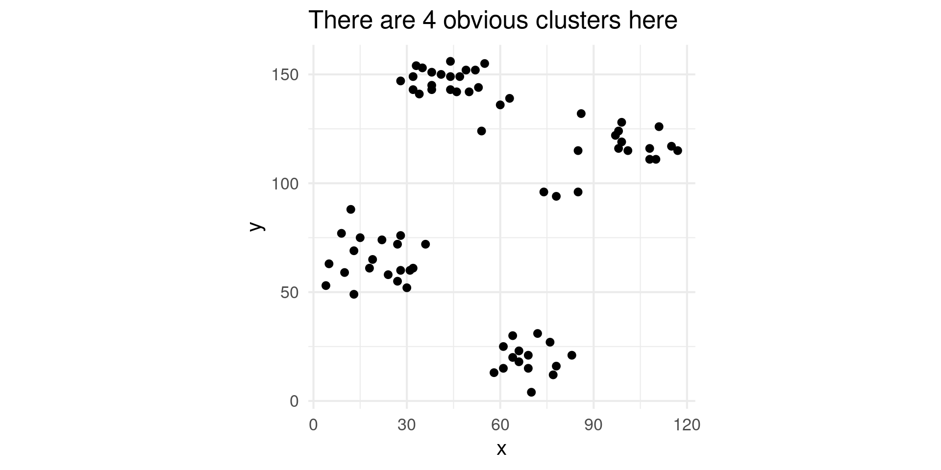
How many clusters?

3 Clusters

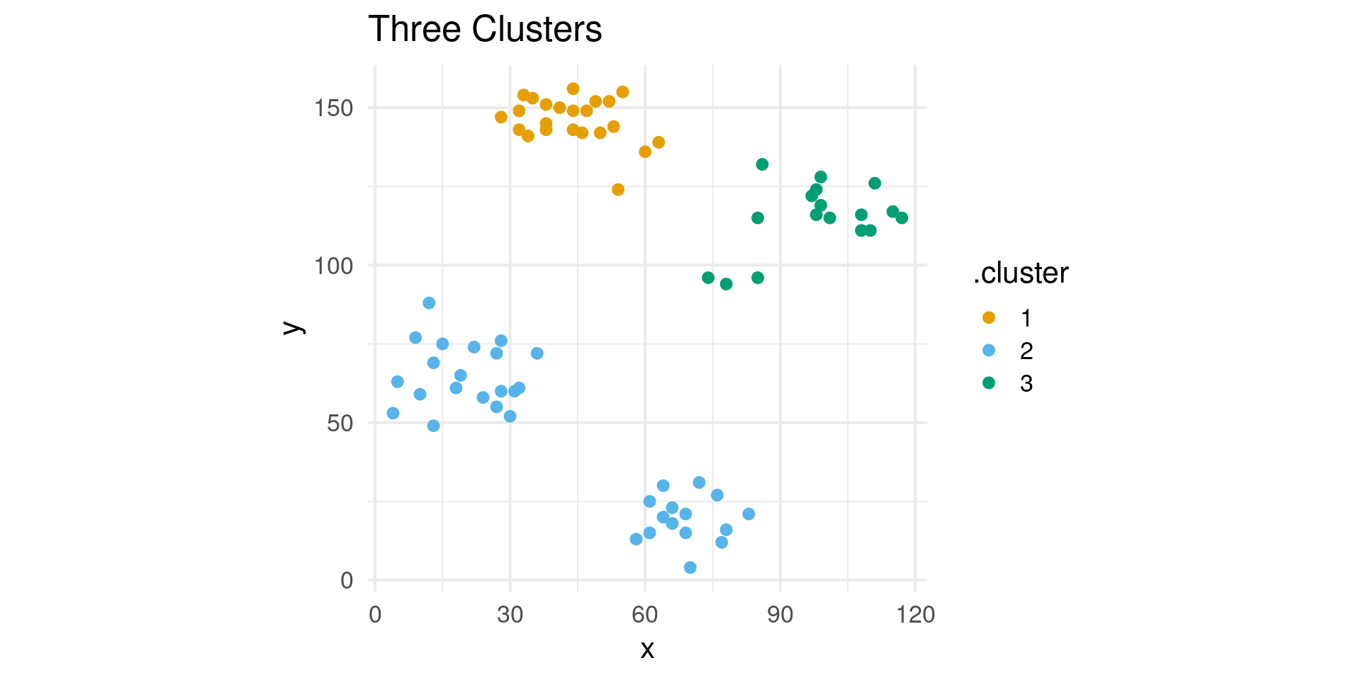
How many clusters?

4 Clusters

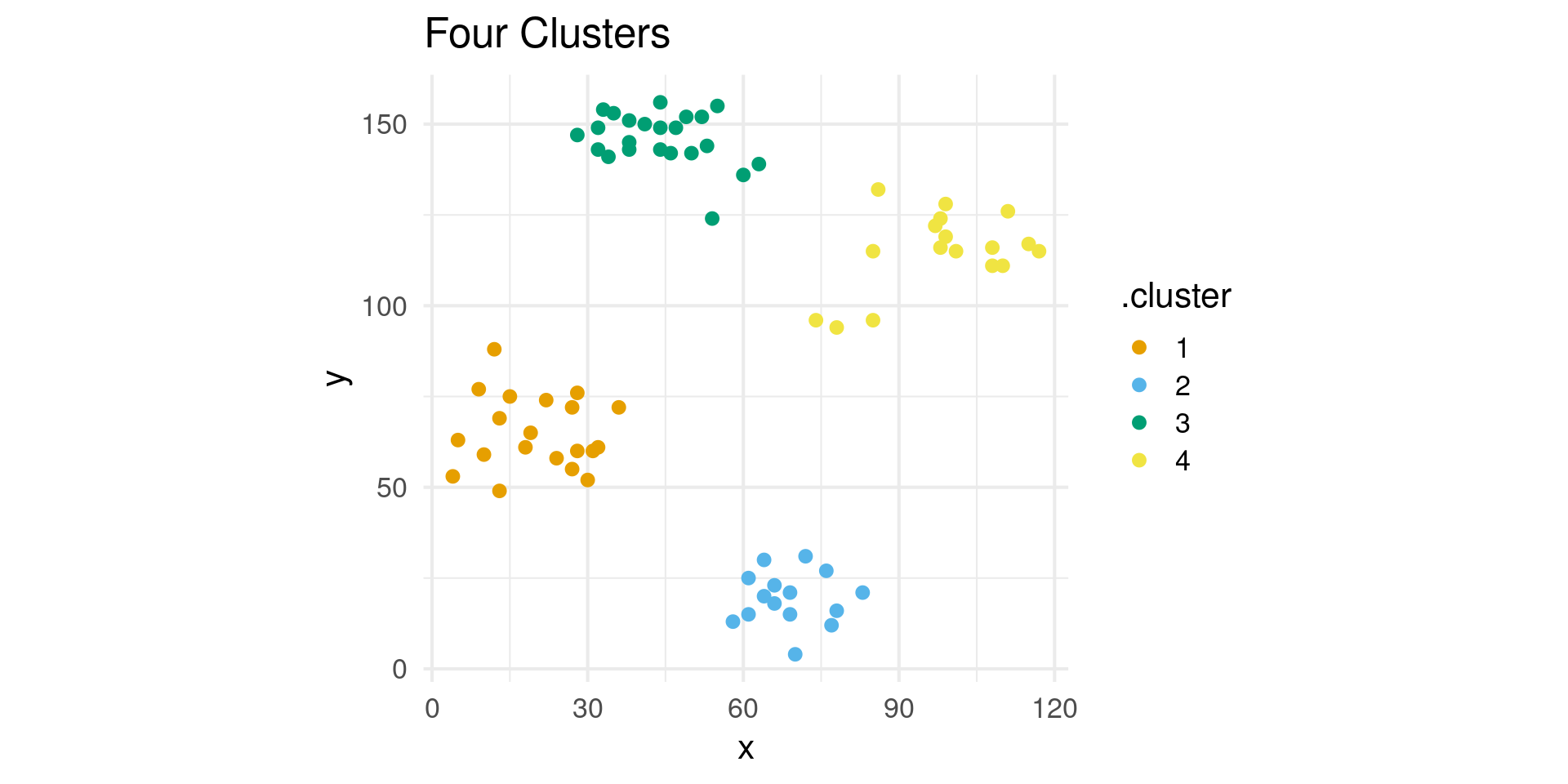
How many clusters?

5 Clusters

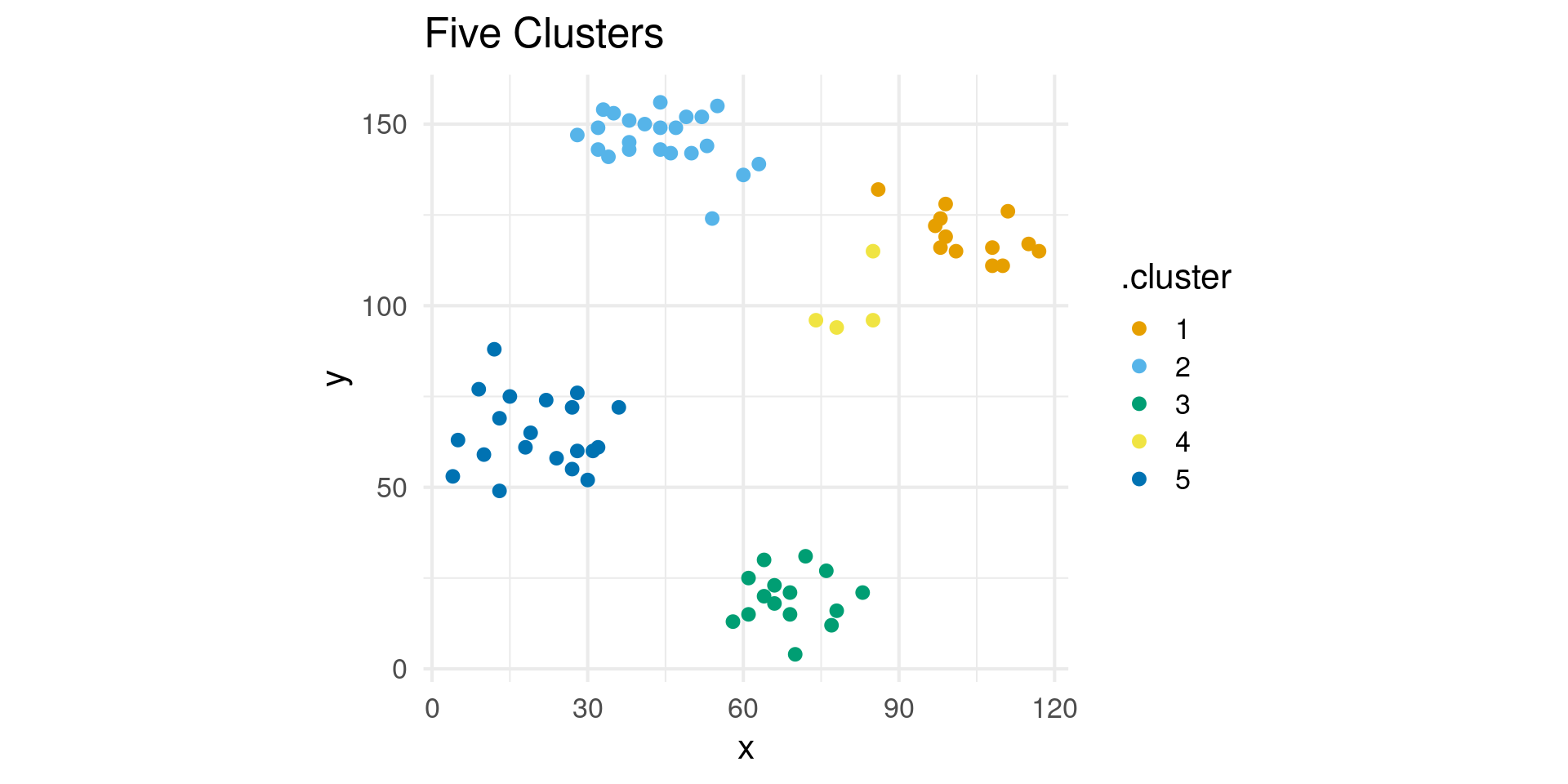
How many clusters?

10 Clusters

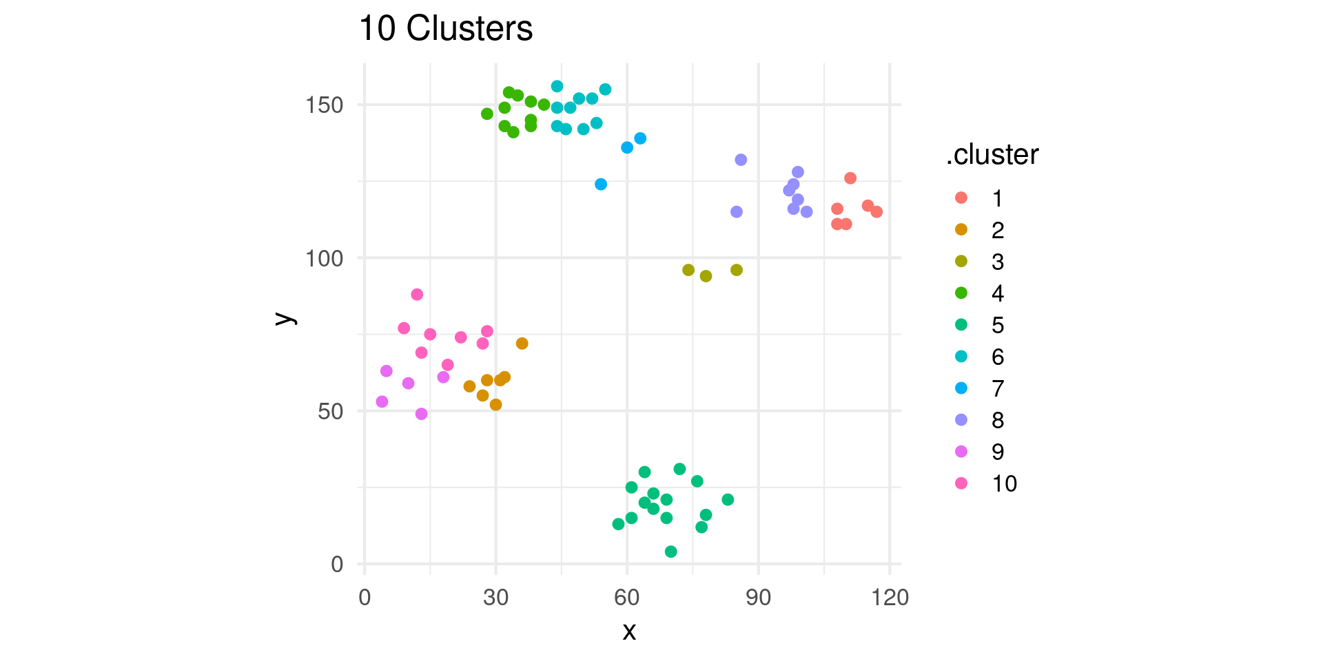
Quantitative Tools for Cluster Number

Many methods for choosing the number of clusters!
Elbow method: Look for elbow in plot of within cluster variance

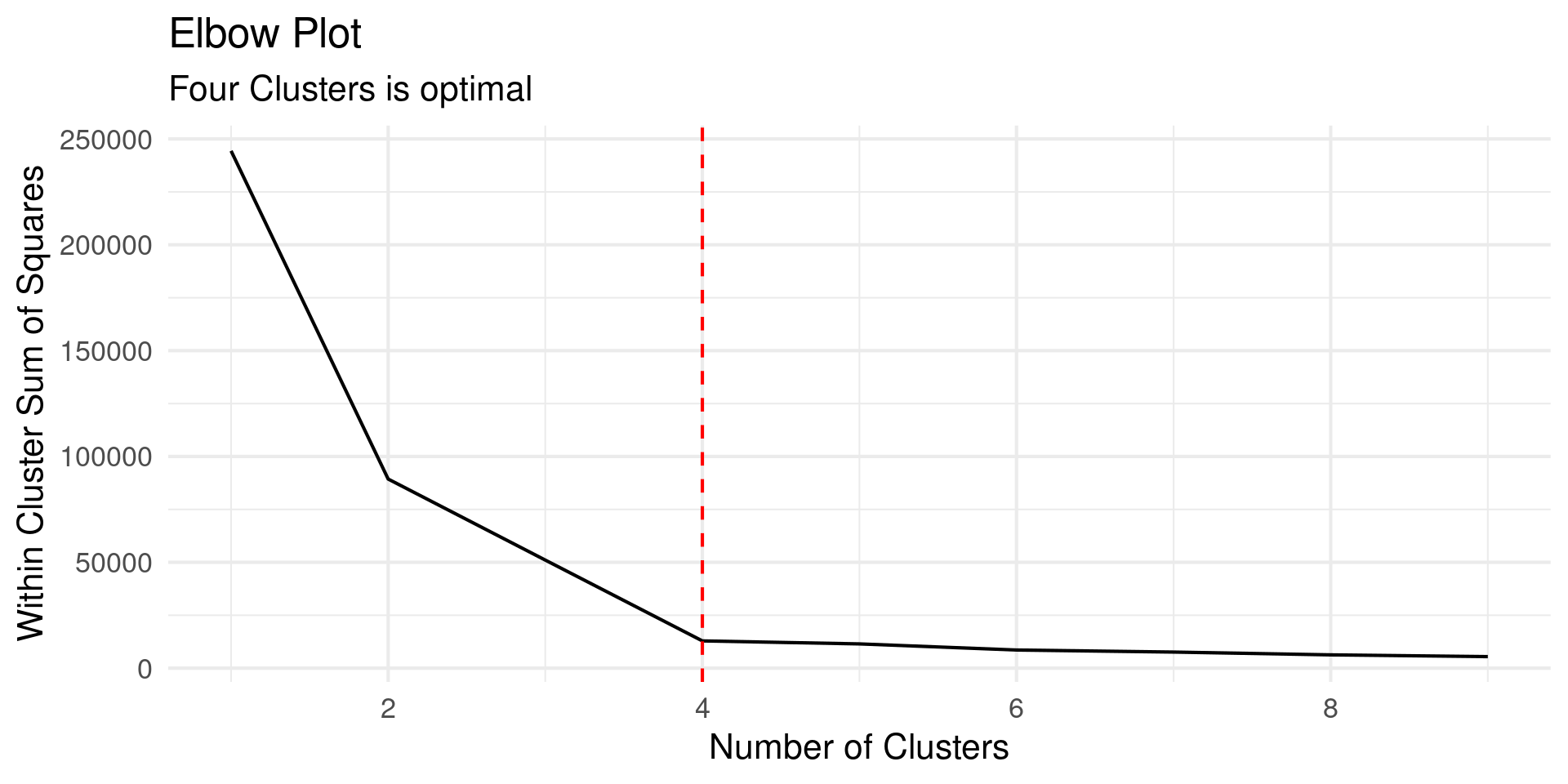
Quantitative Tools for Cluster Number

Many methods for choosing the number of clusters!
Elbow method: Look for elbow in plot of within cluster variance

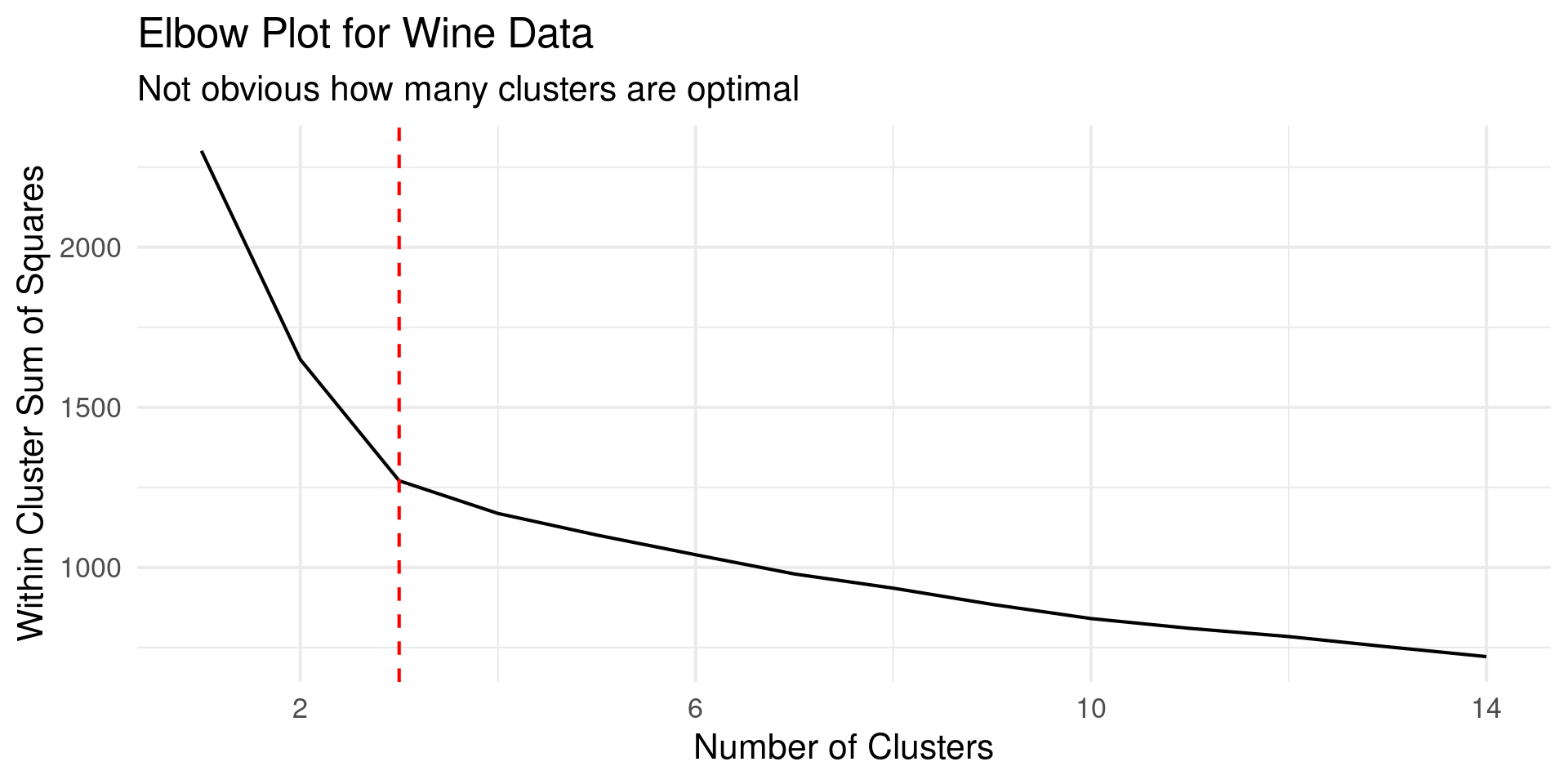
Quantitative Tools for Cluster Number

Use map to apply k-means to many times

kvec = seq(2:10)

wcss = map(kvec,.f = function(k) {
    kmeans(ruspini, centers = k, nstart = 5)$tot.withinss
})
elbow_plot = tibble(clusters = kvec, wcss = wcss) |> unnest()
elbow_plot |> ggplot(aes(kvec, wcss)) + 
  geom_line() +
  geom_vline(xintercept = 4, color = "red", linetype = 2) +
  theme_minimal(base_size = 16) +
  scale_x_continuous(breaks=c(2,4,6,8,10)) +
  labs(title = "Elbow Plot",
       subtitle = "Four Clusters is optimal",
       y = "Within Cluster Sum of Squares",
       x = "Number of Clusters")

Interpreting Clusters

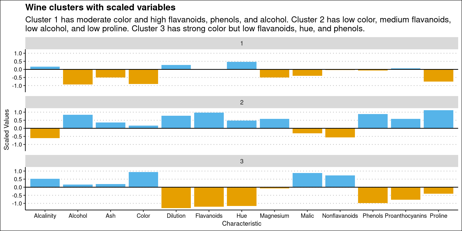
Goal of clustering is often to gain insight.

Interpreting Clusters

Takes some tricky to understand code to transform the PCA coordinates:

wine_df_2 = wine_df |> select(-Type)
centers_df = t(t(wine_clusters$centers %*% t(pca_fit$rotation)) *
            pca_fit$scale + pca_fit$center) |> 
  as_tibble() |> 
  bind_rows(wine_df_2) |> 
  scale() |> 
  as_tibble() |> 
  head(n=3) |>
  mutate(center = seq(1:3))

t(t(wine_clusters$centers %*% t(pca_fit$rotation)) * pca_fit$scale + pca_fit$center) coordinate transformation
scale enables visualization of variables together

Interpreting Clusters

centers_df |> pivot_longer(
  cols = Alcohol:Proline,
  names_to = "type") |> 
  mutate(sign= value>0) |> 
  ggplot(aes(x=type,y=value)) + 
  geom_col(aes(fill=sign)) +
  scale_fill_discrete(guide = "none") +
  geom_hline(yintercept = 0) +
  facet_wrap(~center,nrow=3) +

There could be many ways of visualizing this
Here chose column plot, colored by sign with a horizontal line to denote where 0 is across the facets
I found this a little better than a dot plot for some reason

Annotating Clusters

geom_mark_ellipse to draw circles around clusters

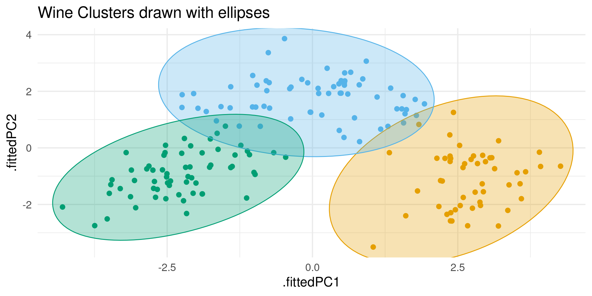
k-means tips and pitfalls

Algorithm not guaranteed to converge
- Can get wrong answes if nstart too low
- Can get stuck in local minima
Very sensitive to outliers and largest scale of data
- Always scale data first or used on scaled coordinates
Assumes Spherical, Balanced Clusters
Will find clusters when there are none

Other Clustering Algorithms

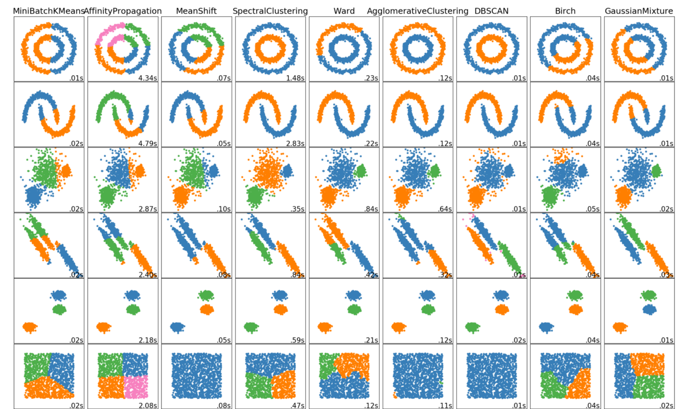
George Seif

DATA 608 Meetup 11: Clustering

Week Summary

Clustering and Dim. Reduction

Clustering and Dim. Reduction

Clustering and Dim. Reduction

Automatic Clustering

k-means method

k-means method

Implementing k-means in R

Key arguments

Key Outputs

Key Outputs

Key Outputs

Key Outputs

How many clusters?

How many clusters?

How many clusters?

How many clusters?

How many clusters?

Quantitative Tools for Cluster Number

Quantitative Tools for Cluster Number

Quantitative Tools for Cluster Number

Interpreting Clusters

Interpreting Clusters

Interpreting Clusters

Annotating Clusters

k-means tips and pitfalls

Other Clustering Algorithms

Thanks!