Meetup 1: Introduction to Optimization
What is Optimization?
- What is the decision that leads to the best outcome?
- What is the value of our decision variable \(\mathbf{x}\) that minimizes our objective function f()?
\[
\textrm{minimize}\quad f(\mathbf{x}), \\
\textrm{subject to}\quad g_i(\mathbf{x}) \leq 0, \\
\textrm{and}\quad h_j(\mathbf{x}) = 0,\\
\mathbf{x}\in \mathbb{R}^n, \quad f,\, g_i,\, h_j: \mathbb{R}^n\mapsto \mathbb{R}
\]
Constraint Terminology
- A feasible point \(\mathbf{x}\) for the optimization problem is a point that satisfies all the constraints: \[
g_i(\mathbf{x}) \leq 0 \\
h_j(\mathbf{x}) = 0
\]
- Technically we don’t need the \(h_j\) terms
- Can get greater than constraints with \(-g_i\)
Optimum Terminology
- \(\mathbf{x}\) is called a local minimum if there is some region \(\Gamma\) surrounding \(\mathbf{x}\) where \(f(\mathbf{x})\leq f(\mathbf{x'})\) for all \(\mathbf{x}'\) in \(\Gamma\).
- \(\mathbf{x}\) is a global minimum if there is no feasible point \(x'\) with \(f(\mathbf{x'})<f(\mathbf{x})\)
- Can turn a maximization problem into a minimization problem by replacing the objective function \(f\) with \(-f\)
Meaning of the math
- \(\mathbf{x}\) represents something we control:
- Coefficients of a linear regression
- Weights of a neural network
- Allocation of $ to advertising channels
- Investment allocations in a portfolio
Meaning of the math
- \(f\) models how the decision \(\mathbf{x}\) impacts us
- RMS error of the regression
- cross-entropy plus a penalty for the weights
- Ad impressions on target demographic
- Expected variance of your portfolio
Meaning of the math
- \(g_i\) and \(h_j\) constrain your decisions \(\mathbf{x}\) so they are realistic
- Can’t put negative $ in an ad channel
- Regulatory limits on leverage, short positions
- Valid probability distribution
- Prior constraints on parameters
Optimization underlies nearly all data science algorithms
Going in depth brings some benefits:
- Recognize what problem you are facing, can enable you to solve it 1000 times easier in some cases
- Understand how the tools you use work and what can go wrong
- Absolutely indispensable for some cutting edge methods (i.e. deep learning)
- Useful non-stats applications
Examples: Least Squares
\(i\)th observation is vector \(\mathbf{a}_i\)
Obs of target function \(b_i\)
Linear model \(b \sim a^t x\)
\[
\textrm{minimize RMS error:}\quad \min_{x\in\mathbb{R}^n} \sum_{i} \left(\mathbf{a}_i^t \mathbf{x}-b_i\right)^2 \] or let \(A\) be the matrix whose rows are the vectors \(\mathbf{a}_i^t\): \[\min_{\mathbf{x}\in\mathbb{R}^n} \|A\mathbf{x}-\mathbf{b}\|^2 \]
Examples: Least Squares
Add penalty terms for regularization or constraints
\[ \min_{\mathbf{x}\in\mathbb{R}^n} \|A\mathbf{x}-\mathbf{b}\|^2 +k\|x\|^2 \\
g_i(\mathbf{x}) \leq 0 \\
h_j(\mathbf{x}) = 0
\]
Examples: Maximum Likelihood
- \(p(\mathbf{y}|\mathbf{x})\) is likelihood of data given parameters
- maximum likelihood is the optimization problem
\[
\textrm{find:}\quad \min_{\mathbf{x}\in\mathbb{R}^n} -\log\left(p(\mathbf{y}|\mathbf{x})\right) \\
\textrm{subject to:}\quad g_i(\mathbf{x}) \leq 0 \\
\textrm{and:}\quad h_j(\mathbf{x}) = 0
\]
Example: Deep Learning
\[ \min_w \sum_i C(\phi(\mathbf{x}_i,\mathbf{w}),y_i), \]
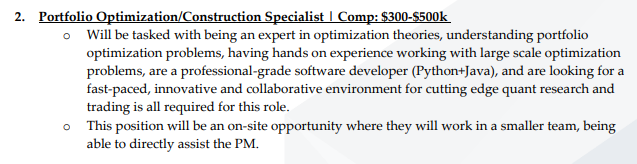
Optimization outside data sciece
![]()
Course Structure
- Least Squares
- Oldest, easiest, most mature technologies, first four weeks
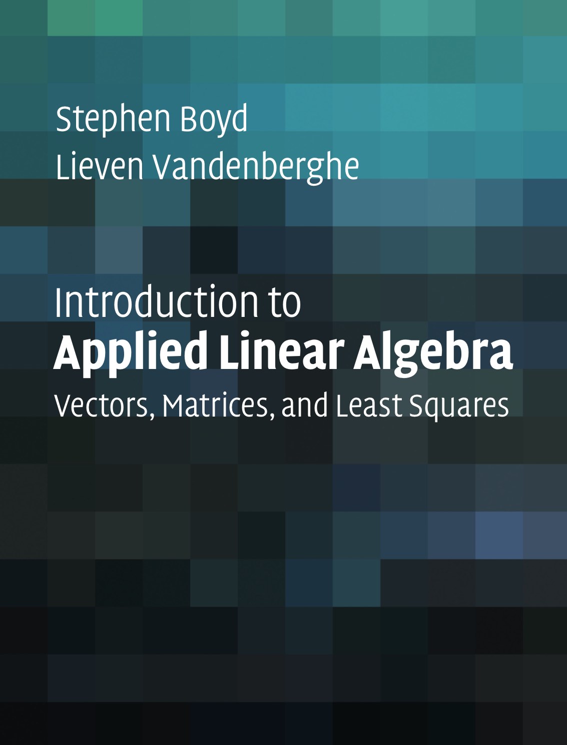
- Primary book is VMLS
Course Structure
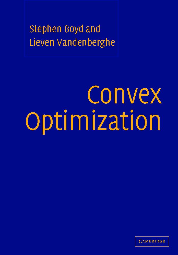
- Convex Optimization
- Non-negative curvature
- Incredibly useful, difficult, weeks 5-12
- Subsumes many special cases (least squares, linear programs, etc)
- Growing field, especially with advent of AI
Other Textbook
- We have one more good book, unforunately not free
- Also doesn’t cover anything in depth
- Great for overall picture
Homework Assignments
- Due every two weeks
- Mostly solving problems with data but some math
- Preferred format: quarto file accompanied with rendered pdf
- Choice of language, Recommended python, Julia, R
- 80% of your grade
Final Project
- Final Project will be to explore an aspect of the course in a little more depth.
- Intentionally open ended, but could be as simple as picking an application area of interest to you and designing and solving a problem in that area
- 20% of your grade
Course Website and Slack Channel
Generative AI Policy
- AI is useful, you can ask it questions, have it generate code, etc
- It is great at easy problems, but that is a trap
- It makes lots of mistakes
- Research shows it helps people who know the material well much more than those who don’t
- Policy: You should understand everything that you turn in completely. I’ll will be generous with grades for genuine effort but will penalize AI-driven mistakes harshly
What to do this week?
Chapter 1 Introduction to Algorithms for Data Mining and Machine Learning
Chapter 1 of Convex Optimization
If needed review linear algebra:
Start Lab 1
- Problem 1 this week, 2 and 3 next week
Optimization: Needles in a haystack?
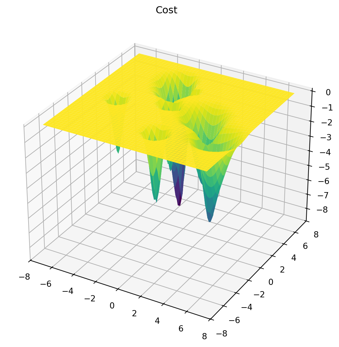
- General optimization is a hard problem
- Error proportional to # boxes sampled: \[\mathrm{Num Boxes} \sim \frac{C}{\epsilon^N}\]
- N is num. parameters
- Modest N, problem takes longer than age of universe
Only Local Optimization is Possible
- Can’t find lowest valley, but can find a valley
- Often, this is still very useful in practice
- No guarantees, sensitive to initial guess
- For convex problems, only one valley!
What is a local minimum?
- value \(\mathbf{x}_0\) where \(f(\mathbf{x})>f(\mathbf{x}_0)\) close
What is a local minimum?
- value \(\mathbf{x}_0\) where \(f(\mathbf{x})>f(\mathbf{x}_0)\) close
- In calculus need two things: \[
\frac{df}{dx} = 0,
\frac{d^2f}{dx^2} > 0
\]
- Function is “flat”
- Curvature is “up”
What is a local minimum?
- value \(\mathbf{x}_0\) where \(f(\mathbf{x})>f(\mathbf{x}_0)\) close
- Higher dimensions \[
\nabla f(\mathbf{x}) = 0 \\
(\nabla^2 f)_{ij} = \frac{\partial^2 f(\mathbf{x})}{\partial x_i \partial x_j} \succ 0
\]
- Vanishing gradient
- Positive Definite “Hessian”
How to find local minimum in practice?
- Iterative methods:
- Gradient Descent, Newton’s Method, ….
- Start with initial guess \(\mathbf{x}_0\)
- Calculate gradient \(\nabla f\)
- Take a “step” in direction of \(\nabla f\) \[ \mathbf{x}_{n+1} = \mathbf{x}_n - k\nabla f(\mathbf{x}_{n})\]
- \(k\) is step size or learning rate
How to find local minimum in practice?
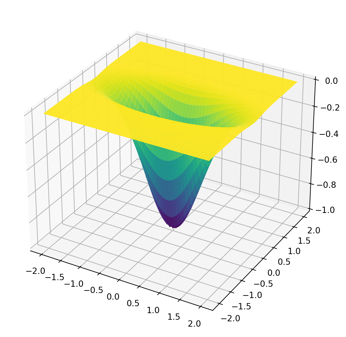
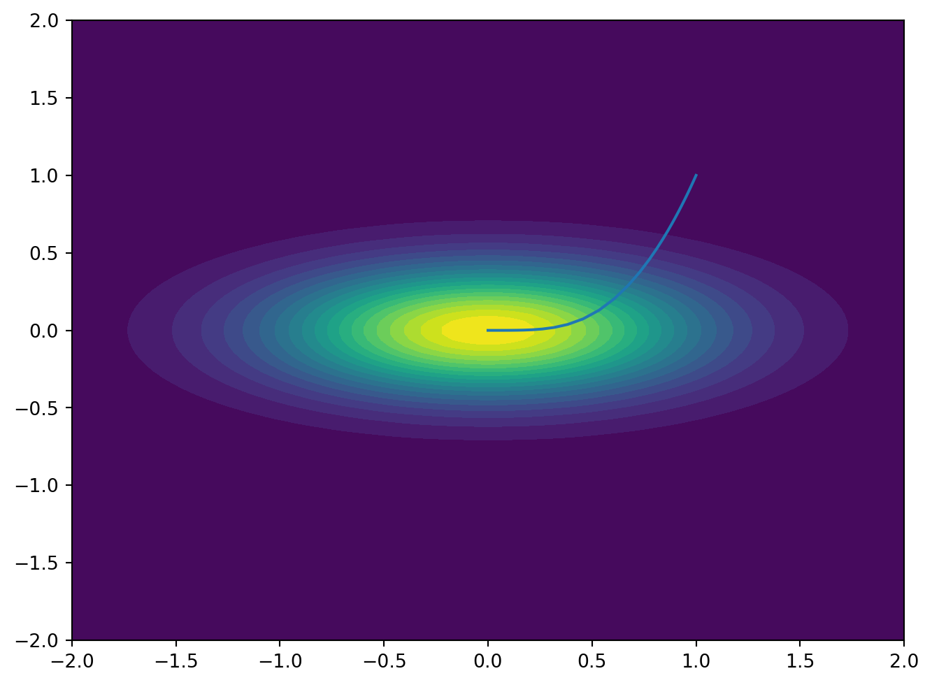
- \(f(x,y) = \exp\left(-x^2-3y^2\right)\)
- \(k=0.1\)
- 100 steps
Advert
- Once per month (Tuesday, Wedneday, Thursday) “field trips” to New York Open Statistical Computing Meetup
- Send me a DM I’ll add you to the email list
- nyhackr.org
![]()