DATA 609 Meetup 11: Application to Statistics and Machine Learning

George I. Hagstrom

Week Summary

Spring Break Next week
HW Due in the week after spring break
Reading: 7.1, 7.2, 8.6
I’ll read your proposals and give some quick feedback

NY Open Statistical Computing Meetup

April 8th 6:30-8:30+
Great Networking/Learning Opportunity

Parametric Statistics

Parametric statistical models assume data generated by a probability distribution that depends on parameters
- Linear regression: \[ y_i| \sim \mathrm{Normal}(\theta^T\mathbf{x}_i + y_0,\sigma) \]
- Here the parameters are \(\theta\), \(y_0\), and \(\sigma\)

Maximum Likelihood

Likelihood is probability of observations given model coefficients \[ p(\mathbf{y}|\theta,\mathbf{x}) = \prod_{i=1}^n p(y_i|\theta,\mathbf{x}_i) \]
Usually work with \(l(\mathbf{y},\mathbf{\theta}) = \log(p(\mathbf{y}|\theta,\mathbf{x}))\): \[ l(\mathbf{y},\theta) = \sum_{i=1}^n \log(p(y_i|\theta,\mathbf{x}_i)) \]

Maximum Likelihood

If \(p\) is a log-concave in \(\theta\) for fixed \(\mathbf{y}\), \(\mathbf{x}\), maximum likelihood is a convex optimization problem:

\[ \mathrm{min}_{\theta}\, -\sum_{i=1}^n \log(p(y_i|\theta,\mathbf{x}_i)) \]

If \(p\) is a log-concave function of \(\theta\), MLE problem is convex

Link to Penalty Functions

Last lecture: \[ \min_{\theta} \sum_{i=1}^n \phi(x,\theta) \]
Here \(\phi(\theta) = \log(p(y_i|\theta,\mathbf{x}_i))\)
Each penalty corresponds to a probability model \[ p(x|\theta) = \frac{e^{-\phi(x,\theta)}}{\int dx' e^{-\phi(x',\theta)}} \]

Probability and Penalty

Squared Residuals corresponds to Gaussian Noise
- \(p(y) = \frac{e^{-y^2/(2\sigma^2)}}{\sqrt{2\pi\sigma^2}}\)
Sum of absolute value of residuals (\(L_1\)) corresponds to Laplace noise:
- \(p(y) = \frac{e^{-|y|/a}}{2a}\)

Convexity of MLE

For Gaussian: \[ -l(\theta) = \left(\frac{n}{2}\right)\log(2\pi\sigma^2) + \frac{\| \theta^T X -\mathbf{y}\|^2}{2\sigma^2} \]
Not convex except if \(\sigma\) fixed
If \(\theta\) is fixed is convex in \(1/\sigma^2\)
Can generalize to covariance estimation

Covariance Estimation

Hard example in 7.1
Have many \(\mathbf{x}_i\) of variables, want to estimate covariance under a normal model \[ -l(\Sigma) = \frac{N}{2}\log(\mathrm{det}\Sigma) + \frac{1}{2}\sum_{i=1}^N \mathbf{x}_i^T\Sigma^{-1}\mathbf{x}_i \]
Only convex in variable \(S = \Sigma^{-1}\)

Prior Knowledge

Can incorporate constraints on parameters as a type of prior knowledge
For example, if the parameters had been previously estimated to within a given accuracy
For example, trying to learn if a coin is fair or not, \(p_1\) is probability of heads
- \(p_1 \sim \mathrm{Beta}(5,5)\)
- You think coin might not be fair

MAP Estimation

Can take prior idea even further and start with a Bayesian model
Observations \(y\) and model parameters \(\theta\)
\(p(\theta|y)\) is probability of parameters \(\theta\) given observations \(y\)
Probability model: \(p(y|\theta)\)
Also have prior beliefs \(p(\theta)\)
Bayes Theorem: \[ p(x|y) = \frac{p(y|\theta)p(\theta)}{p(y)} \]

MAP Estimation

Harder problem: Calculate samples of posterior \(p(\theta|y)\)
Simpler problem: Find value of \(\theta\) that maximimizes \(p(\theta,y)\)
Maximum a-Posteriori Probability: \[ \mathrm{max}_{\theta}\, p(y|\theta)p(\theta) \]

MAP Estimation

Can take log \[ \mathrm{max}_{\theta}\,\, \log\left(p(y|\theta)\right) +\log\left(p(\theta)\right) \]
If \(p(y|\theta)\) and \(p(\theta)\) are log-concave, can solve
Equivalent to maximum likelihood if prior is flat
Prior looks like a regularization term

Non-Parametric Discrete

Consider an unknown probability distribution \(p_i\) over random variable \(X\) with values \(x_i\)
Observable/Feature is a function \(f\) of \(x_i\)
\(Ef(X) = \sum_i f(x_i)p_i\) describes a convex set
- Mean, Variance, probability greater than a threshold

Entropy

Entropy of a distribution/RV is defined as: \[ H(X) = E(-\log(p(x))) = \sum_i -p_i\log(p_i) \]
Convex in \(p_i\)s
Entropy stands for the amount of uncertainty contained in the random variable \(X\)

Maximum Entropy

Suppose you have some measurements/knowledge about a random variable \(X\)
- Could be from expected values of observables
- \(Ef_k(X) = y_k\)
Maximum Entropy probability distribution:

\[ \mathrm{min}_{p_i} \sum_i p_i\log(p_i) \\ \sum_{i} f_k(x_i)p_i = y_k \]

Maximum Entropy in Practice

Enormously useful modeling framework
Application uses ideas from convex optimization
Converts from measurements to prediction while adding least additional information \[ p(x) = \exp\left(\sum_{i} \lambda_i f_i(x)\right) \\ \mathrm{min}_{\lambda} -\sum_i a_i \lambda_i + \int dx p(x|\lambda) \]

KL Divergence

Suppose you have two probability distributions \(p\) and \(q\)
The “surprise” we experience when we use \(q\) as a model for a process driven by \(p\) is given by the KL-Divergence: \[ DL(p||q) = \sum_i p_i \log(p_i/q_i) \]
Common tool used for model comparison
- Imagine \(p_i\) is true distribution
Convex loss function used in machine learning

Classification

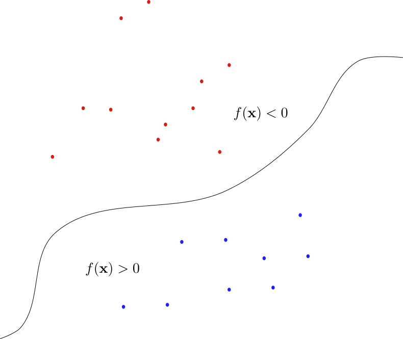
Have two sets of points \(A = \{\mathbf{x}_{a1}, \mathbf{x}_{a2}, \mathbf{x}_{a3}, \dots\}\) and \(B = \{\mathbf{x}_{b1}, \mathbf{x}_{b2}, \mathbf{x}_{b3}, \dots\}\)
Want to find a function \(f:\mathbb{R}^n\to\mathbb{R}\) that satisfies: \[ f(\mathbf{x}) < 0\,\, \mathrm{if}\,\, \mathbf{x} \in A \\ f(\mathbf{x}) > 0\,\, \mathrm{if}\,\, \mathbf{x} \in B \]

Classification

Such an \(f\) classifies or discriminates the points of \(A\) and \(B\)

Classification

To solve classification problem you need a hypothesis set \(\mathcal{H}\) of functions \(f\)
If \(\mathcal{H}\) too complex for dataset you cannot generalize
- Imagine a family of functions which you can just specify to have any values
Leads us to consider simple families \(f\) initially

Linear Discrimination

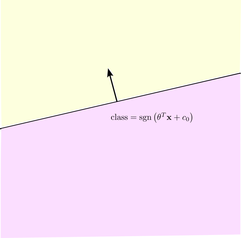
Linear discrimination:
\(f(\mathbf{x}) = \theta^T\mathbf{x} + c_0\)

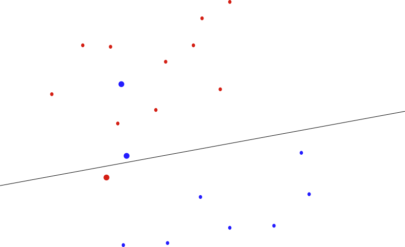
Linear Discrimination Fails

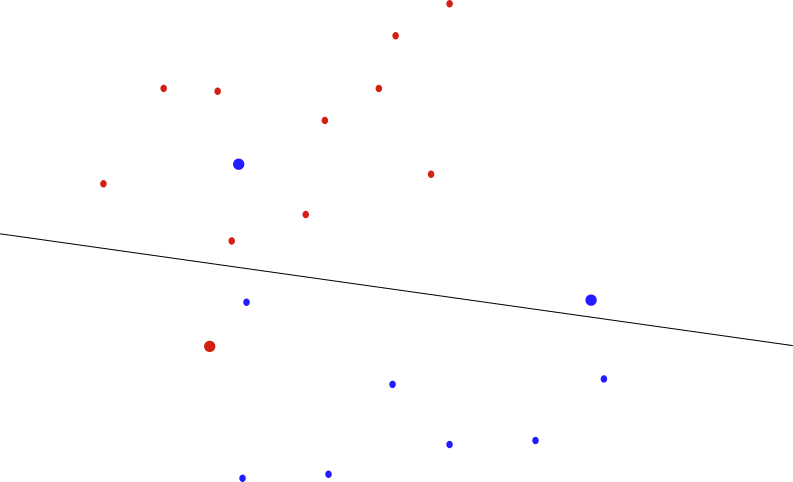
Sets not always linearly separable

Linear Discrimination Fails

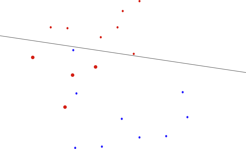
Sets not always linearly separable

Linear Discrimination Fails

Sets not always linearly separable

Linear Discrimination Fails

Need Convex Hull of sets to be disjoint

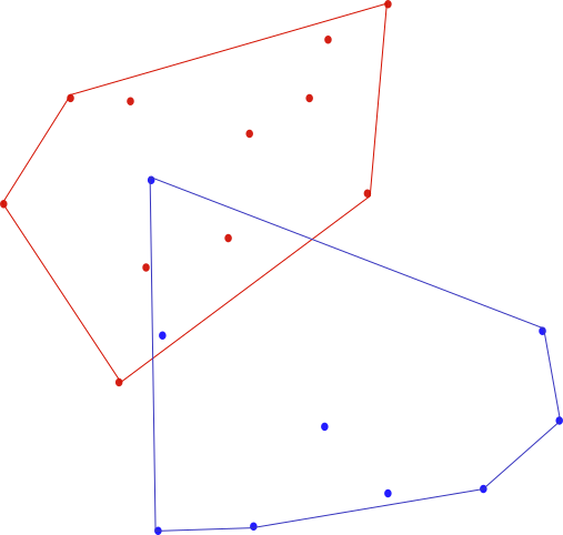
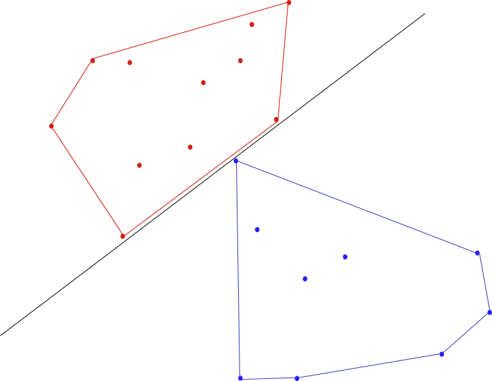
Linear Discrimination Fails

Need Convex Hull of sets to be disjoint

Support Vector Machines

What to do if can’t separate?
Look for approximate separation
- Minimize misclassified points directly is too hard
Instead look to see how bad misclassifications are: \[ \theta^T\mathbf{x}_{ai} + c_0 \geq 1 - u_i \\ \theta^T\mathbf{x}_{bj} + c_0 \leq -(1-v_j) \]
If the \(u_i\) or \(v_j\) are 0, classification successful

SVM Margin

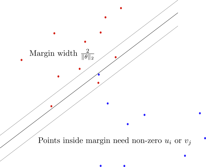
Inequalities create marginal region
Support vectors are points inside

SVM Optimization Problem

Maximize width of slab \(\frac{2}{\|\theta\|_2}\)
- Separates points
Penalize misclassified points
- \(L_1\) norm of \(\mathbf{u}\) and \(\mathbf{v}\)

\[ \mathrm{min}_{\mathbf{u},\mathbf{v},\theta,c_0} \|\theta\|_2+\gamma\left(\mathbf{1}^T\mathbf{u} +\mathbf{1}^T\mathbf{v}\right) \\ \theta^T\mathbf{x}_{ai} + c_0 \geq 1 - u_i\ \\ \theta^T\mathbf{x}_{bj} + c_0 \leq -(1 - v_j)\ \\ \mathbf{u} \succeq 0\,\, \mathbf{v} \succeq 0 \]

SVM Optimization Problem

\[ \mathrm{min}_{\mathbf{u},\mathbf{v},\theta,c_0} \|\theta\|_2+\gamma\left(\mathbf{1}^T\mathbf{u} +\mathbf{1}^T\mathbf{v}\right) \\ \theta^T\mathbf{x}_{ai} + c_0 \geq 1 - u_i\ \\ \theta^T\mathbf{x}_{bj} + c_0 \leq 1 - v_j\ \\ \mathbf{u} \succeq 0\,\, \mathbf{v} \succeq 0 \]

\(\gamma\) balances objective of slab width and misclassified points
Affine plus norm and linear inequalities so convex

Implementation

Reformulate a little
Either \(u_i=0\) or \(u_i = 1-\theta^T\mathbf{x}_{ai}-c_0\)
Either \(v_j=0\) or \(v_j = 1-\theta^T\mathbf{x}_{bj}-c_0\)

\[ \mathrm{min}_{\theta,c_0} \|\theta\|_2 + \gamma\left(\sum_i\mathrm{max}(0,1-\theta^T\mathbf{x}_{ai}-c_0) +\\ \sum_j\mathrm{max}(0,1-\theta^T\mathbf{x}_{bj}-c_0)\right) \]

Implementation

import cvxpy as cp
n = 20
m = 1000
theta = cp.Variable((n,1)) # coefficients
c0 = cp.Variable() # offset
loss = cp.sum(cp.pos(1 - cp.multiply(Y, X @ theta - c0))) # u and v
reg = cp.norm(theta, 1) # width
lambd = cp.Parameter(nonneg=True) # tradeoff
prob = cp.Problem(cp.Minimize(loss/m + lambd*reg)) #

Rescaled loss by number of points
cp.sum(cp.pos(1 - cp.multiply(Y, X @ theta - c0))) is called hinge-loss
\(Y = \pm 1\) is the class

Testing Regularization

# Compute a trade-off curve and record train and test error.
TRIALS = 100
train_error = np.zeros(TRIALS)
test_error = np.zeros(TRIALS)
lambda_vals = np.logspace(-2, 0, TRIALS)
theta_vals = []
for i in range(TRIALS):
    lambd.value = lambda_vals[i]
    prob.solve()
    train_error[i] = (np.sign(X.dot(theta_true) + offset) != np.sign(X.dot(theta.value) - c0.value)).sum()/m
    test_error[i] = (np.sign(X_test.dot(theta_true) + offset) != np.sign(X_test.dot(theta.value) - c0.value)).sum()/TEST
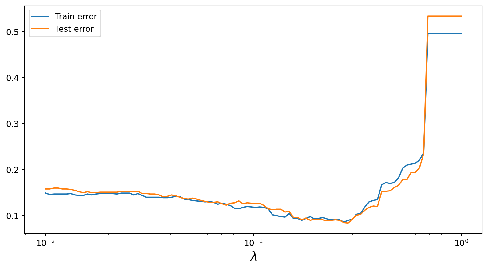
    theta_vals.append(theta.value)

Here test/train errors are percentage of points classified correctly

Train/Test Error

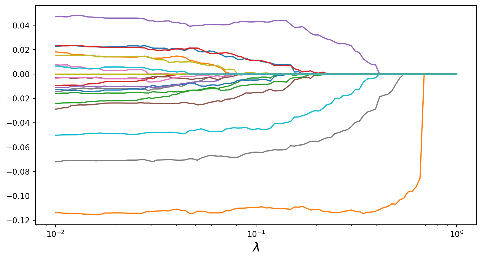
Regularization Paths

for i in range(n):
    plt.plot(lambda_vals, [wi[i,0] for wi in theta_vals])
plt.xlabel(r"$\lambda$", fontsize=16)
plt.xscale("log")

Do more with SVMs

SVMs not restricted to linear separation
Can use nonlinear functions to generate additional features
Leads to higher dimensional space in which sometimes linear separator is more effective

DATA 609 Meetup 11: Application to Statistics and Machine Learning

Week Summary

NY Open Statistical Computing Meetup

Parametric Statistics

Maximum Likelihood

Maximum Likelihood

Link to Penalty Functions

Probability and Penalty

Convexity of MLE

Covariance Estimation

Prior Knowledge

MAP Estimation

MAP Estimation

MAP Estimation

Non-Parametric Discrete

Entropy

Maximum Entropy

Maximum Entropy in Practice

KL Divergence

Classification

Classification

Classification

Linear Discrimination

Linear Discrimination Fails

Linear Discrimination Fails

Linear Discrimination Fails

Linear Discrimination Fails

Linear Discrimination Fails

Support Vector Machines

SVM Margin

SVM Optimization Problem

SVM Optimization Problem

Implementation

Implementation

Testing Regularization

Train/Test Error

Regularization Paths

Do more with SVMs

Thanks!