DATA 609 Meetup 12: Duality

George I. Hagstrom

Week Summary

• This week is about duality
  • Let’s you perform a sensitivity analysis of your optimization problem
  • Enables solution of more difficult problems
• Lab 6 is Due this week at midnight
• Reading is parts of Chapter 5: 5.1, 5.2, 5.4.3, 5.4.4, 5.5.2, 5.6
• If you want, Section 3.3

May 9th Meetup!

What is Duality?

• For every optimization problem (not necessarily convex): \[ \mathrm{min}_{\mathbf{x}} f(\mathbf{x}),\quad g_i(\mathbf{x}) \leq 0,\quad h_j(\mathbf{x}) = 0 \]
• There is a “dual” optimization problem: \[ \min_{(\lambda,\nu)} f_d(\lambda,\nu),\quad \lambda_i \geq 0 \]
• The dual variables correspond to constraints and have interpretation as prices
• \(f_d\) depends on original objective and constraints

Why do we care about duality?

• The dual problem is always convex!
• The dual will provide a lower bound on the original objective
• For convex problems, the dual problem is equivalent*
• The dual tells us how the solution changes when we change our problem

Economic perspective on dual

• Consider original problem with inequality constraints: \[ \mathrm{min}_{\mathbf{x}} f(\mathbf{x}),\quad g_i(\mathbf{x}) \leq 0 \]
• Suppose \(f(\mathbf{x})\) was the “profit” of our organization
• \(g_i(\mathbf{x})\) constraint represents capacity constraint:
  • \(g\) could be our available warehouse space
  • \(g\) could be how many employees we have
  • \(g\) could be our freight capacity

Attach a cost to constraint

• Suppose we could pay a cost \(\lambda\) to get more warehouse space/freight capacity/employees: \[ \mathrm{min}_{\mathbf{x}} f(\mathbf{x}) + \lambda g(\mathbf{x}) \]

Attach a cost to constraint

• Alternative optimization problem

\[ \mathrm{min}_{\mathbf{x}} f(\mathbf{x}) + \lambda g(\mathbf{x}) \]

• Suppose that if we don’t use all capacity, we can get some money back
  • renting unused warehouse space,
  • selling freight capacity
  • reducing headcount

Multiple Constraints

• If we have multiple constraints, each one has a lambda: \[ \min_{x}f(\mathbf{x}) + \sum_{i}\lambda_i g_i(\mathbf{x}) \]

Lagrange Dual

• Let \(f_d(\lambda) = \min_{\mathbf{x}}f(\mathbf{x}) + \lambda g(\mathbf{x})\)
• \(f_d(\lambda)\) is the optimal profit for a given cost \(\lambda\)
• \(f_d(\lambda)\) is a concave function of \(\lambda\)
• \(f_d(\lambda)\) is called the Lagrange Dual function of the optimization problem
  
• Soon will generalize it to equality constraints

Lower bound on original problem

• Let \(p^{\star}\) be the solution of original problem: \[ p^{\star} = \mathrm{min}_{\mathbf{x}} f(\mathbf{x}),\quad g(\mathbf{x})\leq 0 \]

• Let \(\mathbf{x}^{\star}\) be the value of the decision variables at the minimum \[ p^{\star} = f(\mathbf{x}^{\star}) \geq \cdots\\ f(\mathbf{x}^{\star}) + \lambda g(\mathbf{x}^{\star}) \geq f_d(\lambda) \]

• Lagrange dual for any value of \(\lambda\) is a lower bound on original (aka primal) problem

Generalization to equality constraints

• For inequality constraints, \(\lambda \geq 0\)
• For equality constraints, multiply by \(\nu\): \[ f_d(\lambda,\nu) = \min_{\mathbf{x}} f(\mathbf{x}) +\sum_{i}\lambda_i g_i(\mathbf{x}) + \sum_j \nu_j h_j(\mathbf{x}) \]
• Intuition: equality constraint is like inequality constraint for \(h\) and \(-h\).
• \(\nu\) can have either sign

Lagrangian Function

• Theory of Lagrange Multipliers: \[ L(\mathbf{x},\lambda,\nu) = f(\mathbf{x}) +\sum_{i}\lambda_i g_i(\mathbf{x}) + \sum_j \nu_j h_j(\mathbf{x}) \]
• This is called the Lagrangian function

Dual Optimization Problem

• If \(f_d(\lambda,\nu)\) provides a lower bound on the optimal value of the primal problem, makes sense to find the greatest lower bound
• Dual optimization problem: \[ p^{\star}_d = \max_{(\lambda,\nu)} f_d(\lambda,\nu) \\ \lambda_i \geq 0 \]
• \(f_d\) concave, taking max is analogous to solving a convex optimization problem

Game Interpretation

• Suppose we have a two player game
• Player 1 will choose prices \(\lambda\) and \(\nu\)
• Player 2 then picks action \(x\)
• Goal of Player 2 is to maximize their own profit
• Goal of Player 1 is to minimize Player 2s profit

Game Interpretation

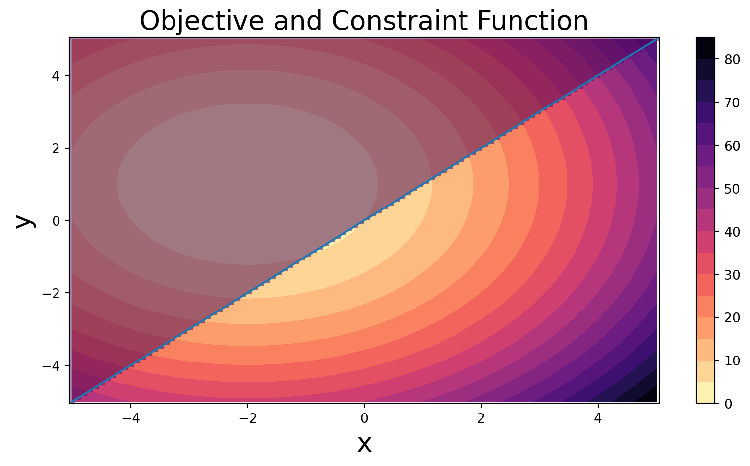
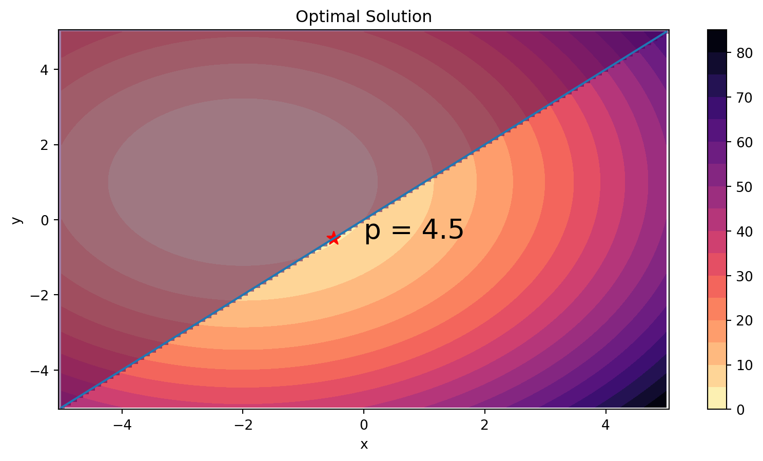
• Consider the following optimization problem \[ \min_{(x,y)} (x+2)^2+(y-1)^2\,\\ x-y \leq 0 \]

Game Interpretation

• Player 2 picks price \(\lambda\)
• Player 1 picks action \(x\) to minimize \[ \min_{(x,y)} ( (x+2)^2 + (y-1)^2 + \lambda(x-y)) \]
• Player 1 wants this function as big as possible
• Player 2 wants this function as small as possible

Game Interpretation

Game Interpretation

Game Interpretation

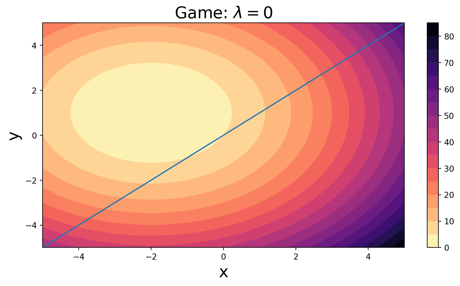
• \(\lambda = 0\)

Game Interpretation

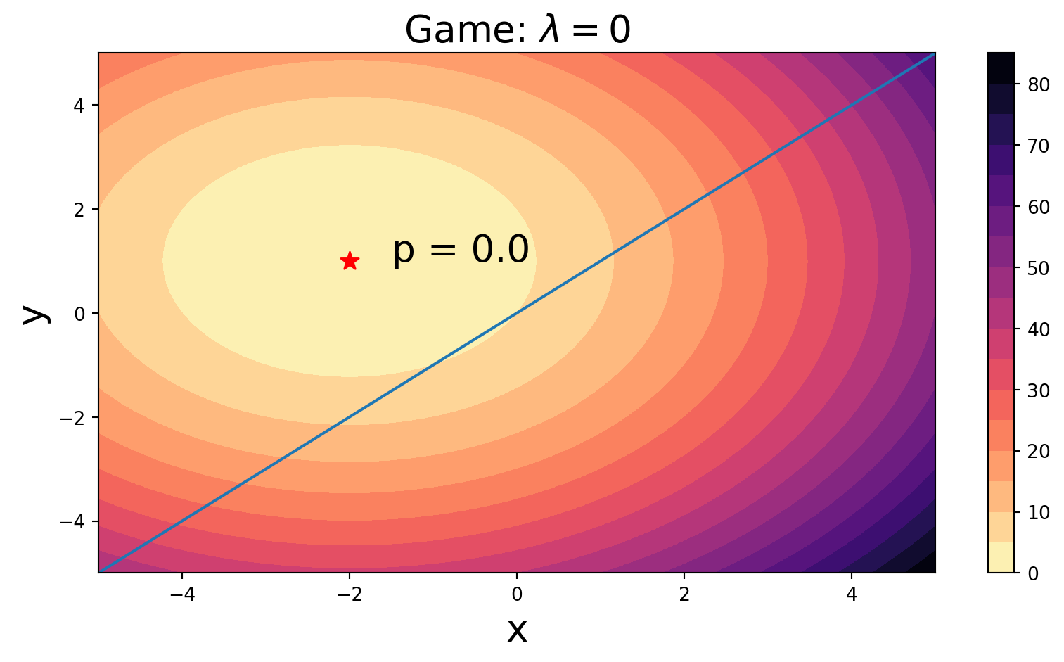
• \(\lambda = 0\)
• \(p=0\)

Game Interpretation

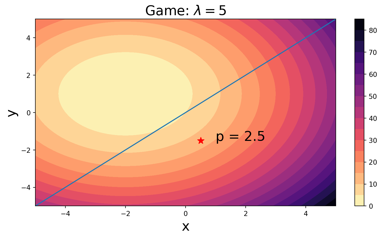
• \(\lambda = 5\)
• \(p=2.5\)

Game Interpretation

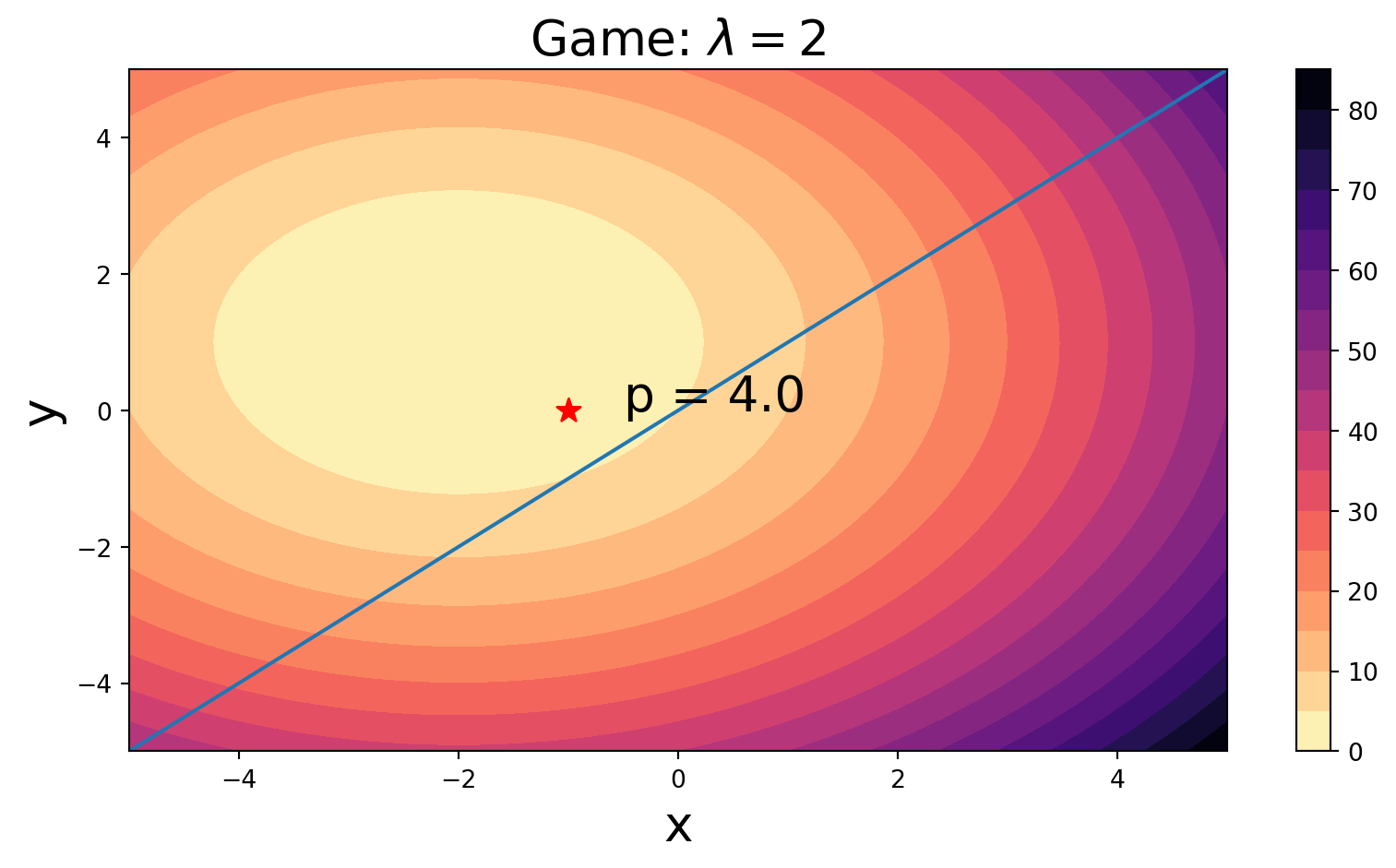
• \(\lambda =2\)
• \(p=4\)

Game Interpretation

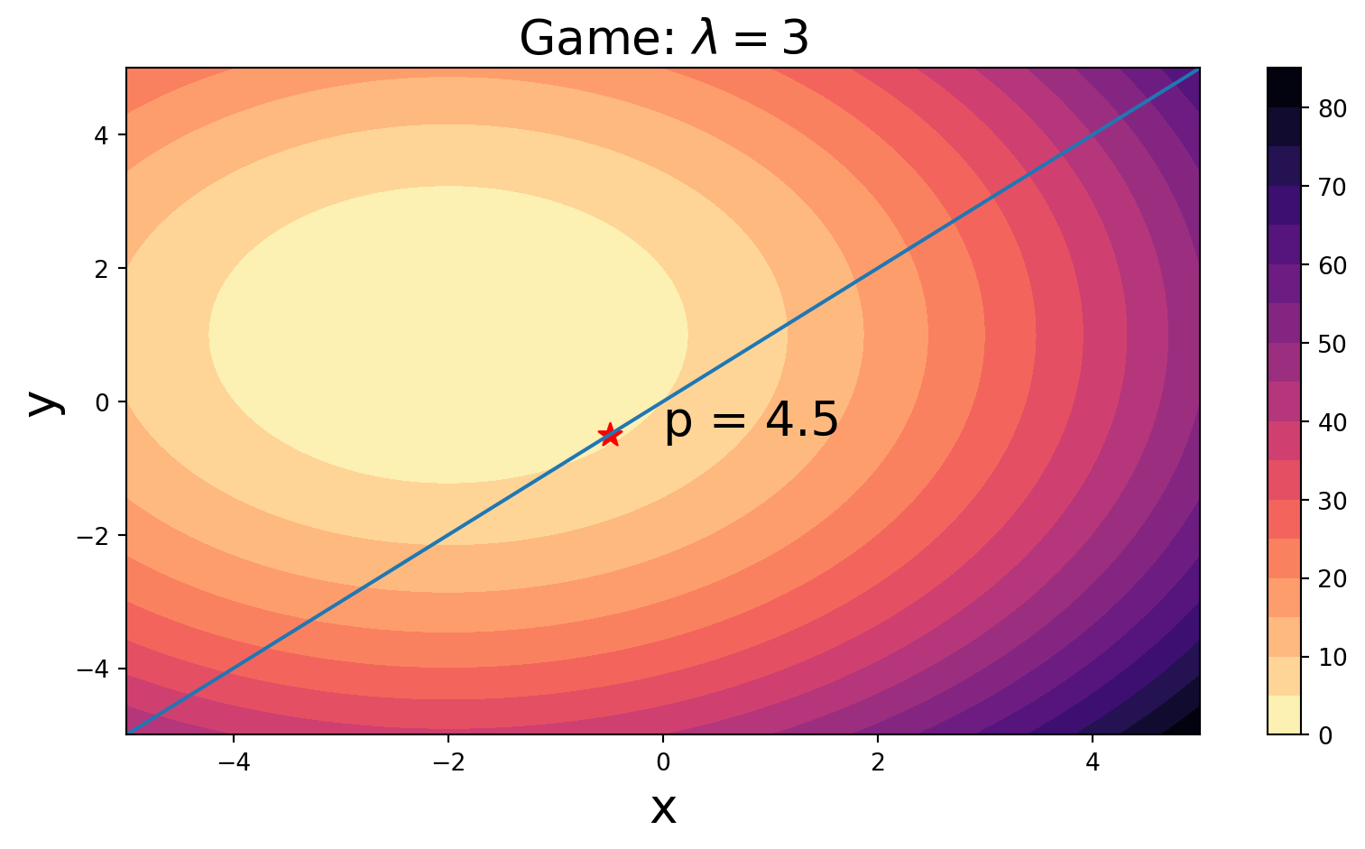
• \(\lambda = 3\)
• \(p=4.5\)
• Maximum
• Min of original prob

Strong Duality

• When original problem is convex, primal and dual problems have same minimum
  • Some rare cases when not true
  • See section on Slater’s Condition
• CVX is a primal/dual solver
  • Simultaneously solves both the primal and dual problem

How to find the dual

• Consider previous problem
• After solving, prob.solution.dual_vars

x_var = cvx.Variable()
y_var = cvx.Variable()

obj = cvx.square(x_var+2) + cvx.square(y_var-1)
constr = -x_var+y_var
prob = cvx.Problem(cvx.Minimize(obj),[constr<=0])
print(prob.solve())
print(prob.solution.dual_vars)

4.5
{248: array(3.)}

Meaning of Dual: Shadow Prices

• Economic Interpretation:
  • Prices \(\mu\) and \(\lambda\) where the firm doesn’t gain from violating constraints
  • Gain in objective from relaxing the constraints: \[ \min_{\mathbf{x}} f(\mathbf{x}) \\ g_i(\mathbf{x}) - u_i \leq 0 \\ h_j(\mathbf{x}) - v_j = 0 \]

Shadow Prices

• Then: \[ \lambda_i = \frac{\partial p^{\star}}{\partial u_i} \\ \mu_j = \frac{\partial p^{\star}}{\partial v_j} \]
• The shadow prices tell us the sensitivity to constraints
• Complimentary Slackness: -\(\lambda_i = 0\) means inequality is inactive

Oil Refining Example

Oil Refining Example

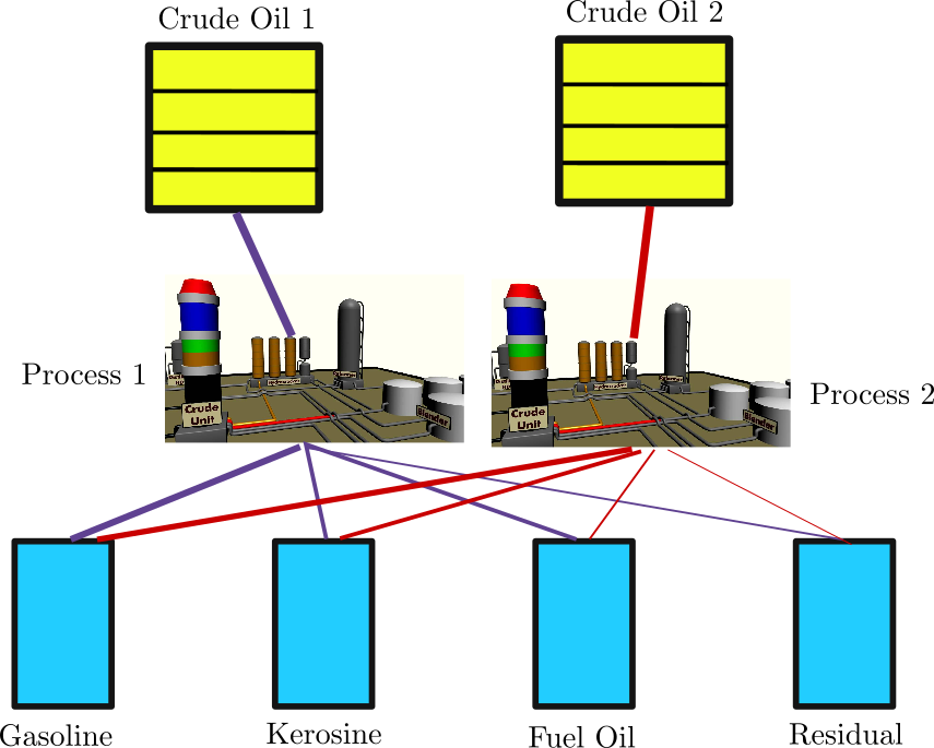
• Two types of crude oil feedstock exist
• Each can be refined
  • Process yields 4 products
  • Process has limit
  • Each product has a limit
• Products and Crude have prices

Oil Refining Example

\[ \max_{\mathbf{c}} \left(\underbrace{\mathbf{p}_{\mathrm{prod}}^T Y\mathbf{c}}_{\mathrm{profit}} -\underbrace{\left(\mathbf{p}_{\mathrm{proc}}^T+\mathbf{p}_{\mathrm{crude}}^T\right)\mathbf{c}}_{\mathrm{costs}} \right) \\ 0\preceq\mathbf{c}\preceq \mathbf{c}_{\mathrm{max}},\quad \mathrm{crude\,\, capacity} \\ 0 \preceq Y\mathbf{c} \preceq \mathbf{L}_{\mathrm{prod}} \]

Oil Refining Products

	capacity	price
gasoline	24000	108
kerosine	2000	72
fuel oil	6000	63
residual	2500	30

Oil Refining Examples

• Crude prices and constraints

	available	price	process_cost
crude 1	28000.0	72.0	1.5
crude 2	15000.0	45.0	3.0

• Process Yields and Costs

	gasoline	kerosine	fuel oil	residual
crude 1	80	5	10	5
crude 2	44	10	36	10

Solving the Problem

# decision variables, this is a vector of length 2
x = cvx.Variable(len(crudes.index), pos=True, name="crudes")

# the objective will be the revenue minus costs

# The production is the amount of each crude times the yield matrix
prods = yields.to_numpy().T @ x / 100.0

# To find revenue we sum up the production times the price of each crude

revenue = products["price"].to_numpy().T @ prods

# Feed costs are the crude prices times the decision variable, summed up
feed_cost = crudes["price"].to_numpy().T @ x

# Ditto for the process costs

process_cost = crudes["process_cost"].to_numpy().T @ x

# profit 

profit = revenue - feed_cost - process_cost
objective = cvx.Maximize(profit)

# constraints: can't use more crude than you have
feeds = x <= crudes["available"].to_numpy()

# Can't produce more of each product than the capacity

capacity = prods <= products["capacity"].to_numpy()

# put them together to get all the constraints

constraints = [feeds, capacity]

# solve using cvx

problem = cvx.Problem(objective, constraints)
problem.solve()

860275.8569415306

Results

• Crude Consumption

	available	price	process_cost	consumption	shadow price
crude 1	28000.0	72.0	1.5	26206.9	0.0
crude 2	15000.0	45.0	3.0	6896.6	0.0

• Product Capacity

	capacity	price	production	unused capacity	shadow price
gasoline	24000	108	24000.0	0.0	14.0
kerosine	2000	72	2000.0	0.0	262.6
fuel oil	6000	63	5103.4	896.6	0.0
residual	2500	30	2000.0	500.0	0.0

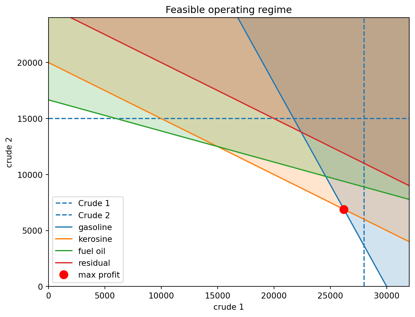
Kerosine Shadow Price

Improving Profits

• In current environment, improve Kerosine capacity
  • Every unit increase in Kerosine adds $262.6 in profit
• What if we doubled Kerosine capacity?
  • Linear estimate is a global upper bound on profit
  • Would be a lower bound for convex
  • Gain is at most 525000

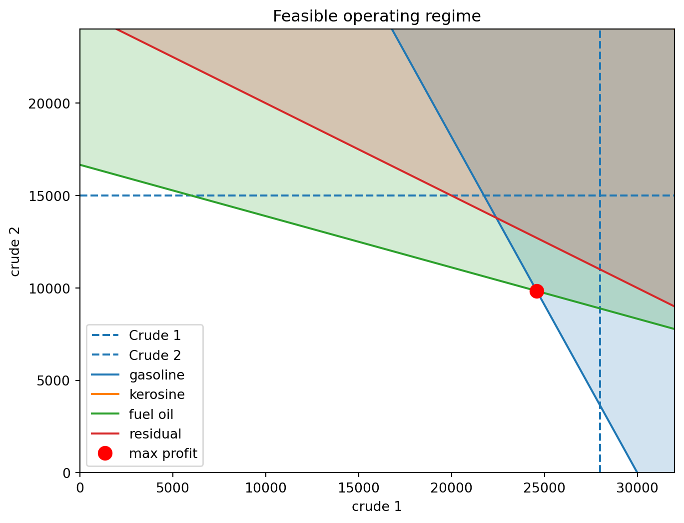
Double Capacity

	available	price	process_cost	consumption	shadow price
crude 1	28000.0	72.0	1.5	24590.2	0.0
crude 2	15000.0	45.0	3.0	9836.1	0.0

	capacity	price	production	unused capacity	shadow price
gasoline	24000	108	24000.0	0.0	22.6
kerosine	4000	72	2213.1	1786.9	0.0
fuel oil	6000	63	6000.0	0.0	62.4
residual	2500	30	2213.1	286.9	0.0

Total Profit:  916229.508181

• Did not reach expected profit target

Double Capacity

Robustness to Shocks

• What if Crude 1 wasn’t available?

crudes = pd.DataFrame(
    {
        "crude 1": {"available": 0, "price": 72, "process_cost": 1.5},
        "crude 2": {"available": 15000, "price": 45, "process_cost": 3},
    }
).T

# constraints
feeds = x <= crudes["available"].to_numpy()
capacity = prods <= products["capacity"].to_numpy()
constraints = [feeds, capacity]

# solution
problem = cvx.Problem(objective, constraints)
problem.solve()

486000.0

Robustness to Shocks

• We are left with tons of spare capacity

	available	price	process_cost	consumption	shadow price
crude 1	0.0	72.0	1.5	0.0	24.3
crude 2	15000.0	45.0	3.0	15000.0	32.4

	capacity	price	production	unused capacity	shadow price
gasoline	24000	108	6600.0	17400.0	0.0
kerosine	4000	72	1500.0	2500.0	0.0
fuel oil	6000	63	5400.0	600.0	0.0
residual	2500	30	1500.0	1000.0	0.0

Capacity Limits?

• If any capacity is cut to 0, profit cut to 0 as well

0.0

• Instead we will see what happens with 80% declines in capacity
• Loop over the four products and study the impact

Resilience to Capacity Shocks

# Initialize products data frame with decline
products["obj_loss"] = 0.0

# Start with a loop over each crude product

for product in products.index:   
  # Make a deep copy of the data
  # This lets us change elements without 
  # overwriting the original data
  products_2 = products.copy()

  # Now we are going to reduce the capacity by 80%
  products_2["capacity"].at[product] = 0.2*products["capacity"].at[product]
  
  # We are ready to solve the optimization problem
  feeds = x <= crudes["available"].to_numpy()
  capacity = prods <= products_2["capacity"].to_numpy()
  constraints = [feeds, capacity]
  # solution
  problem = cvx.Problem(objective, constraints)
  obj = problem.solve()
  # Now we compute the relative decrease and save it
  products["obj_loss"].at[product] = obj/original_obj

Resilience to Capacity Shocks

• Let’s look at the objective declines:

gasoline    0.410862
kerosine    0.225974
fuel oil    0.338961
residual    0.282468
Name: obj_loss, dtype: float64

• Lots of resilience to gasoline capacity loss
  • Interesting since the inequality was active
• Very little resilience to kersoine capacity loss
  • Decrease almost linear in capacity

Can duals be computed?

• So far the dual problem has been abstract
• Involves a minimum function: \[ \max_{(\lambda,\nu)} \min_{\mathbf{x}} L(\mathbf{x},\lambda,\nu) \]
  • Can we ever write out the dual problem explicitly?
    • Sometimes

Dual with Linear Constraints

• Consider an optimization problem with linear constraints: \[ \min_{\mathbf{x}} f(\mathbf{x}) \\ A\mathbf{x} \preceq \mathbf{b} \\ C\mathbf{x} = \mathbf{d} \]
• Dual Objective: \[ \max_{(\lambda,\nu)} \min_{\mathbf{x}}\left( f(\mathbf{x}) + \lambda^T(A\mathbf{x}-\mathbf{b}) + \nu^T\left(C\mathbf{x}-\mathbf{d}\right)\right) \]

Dual and Convex Conjugate

• Can regroup the dual objective: \[ \max_{(\lambda,\nu)}\left( -\lambda^T\mathbf{b} -\nu^T\mathbf{d} +\min_{\mathbf{x}}\left((\lambda^TA+\nu^TC)\mathbf{x}+f(\mathbf{x}) \right) \right) \]
• For some functions \(f\) we can calculate the term inside the minimum
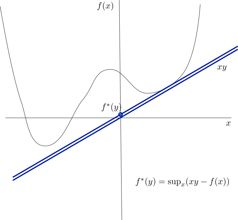
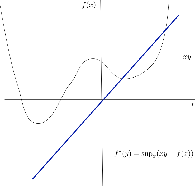
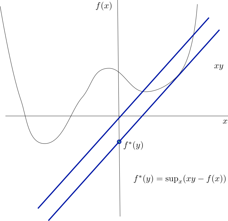
• It is called the convex conjugate of \(f\): \[ f^*(\gamma) = \max_{\mathbf{x}} \gamma^T\mathbf{x} - f(\mathbf{x}) \]

Dual and Convex Conjugate

• In terms of Convex Conjugate \[ \max_{(\lambda,\nu)}-\lambda^T\mathbf{b} -\nu^T\mathbf{d} - f^*(-A^T\lambda-C^T\nu) \\ \lambda \succeq 0 \\ \]

• So if we can compute convex conjugate of objective, can actually write dual problem

Meaning of Convex Conjugate

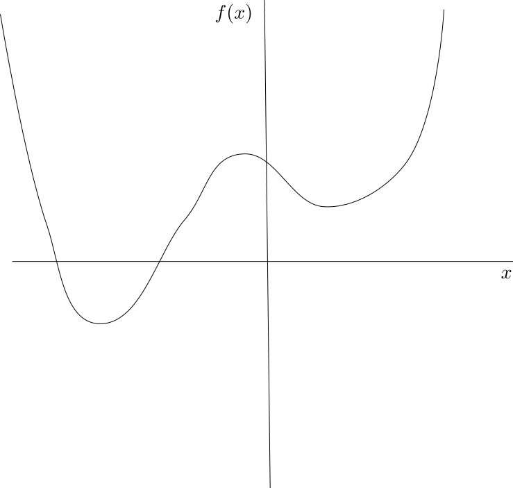
Meaning of Convex Conjugate

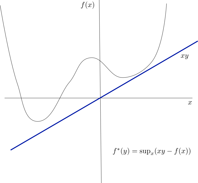
Meaning of Convex Conjugate

Meaning of Convex Conjugate

Meaning of Convex Conjugate

Properties of Convex Conjugate

• It is a convex function
• If \(f\) is convex, \((f^*)^*=f\)
• If function is concave, it is undefined

Convex Conjugate of Some Functions

• Affine Function:
• \(f(x) = ax + b\)
• \(\mathrm{sup}_x (xy - ax - b)\) is infinity unless the \(x\) cancels.
• \(f^*(y)=b\), domain is \(y\in\{a\}\)

Convex Conjugate of Some Functions

• Exponential Function:
• \(f(x) = e^x\)
• \(\mathrm{sup}_x (xy - e^x)\)
• if \(y<0\) this goes to infinity for negative \(x\)
• if \(y>0\) solve equation \(y = e^x\) so \(x=\log(y)\)
• \(f^*(y) = y\log(y) - y\)
• \(f^*(0) = 0\)

Thanks!