Meetup 4: Constrained Least Squares

George I. Hagstrom

Everything in life has constraints

Why can’t you build a car with:
- Speed of Ferrari
- Practicality of minivan

Ferrari Concept

Everything in life has constraints

Size brings weight and poor aerodynamics
Power hurts durability
Cost through the roof

Ferrari Concept

Everything in life has constraints

This theme applies throughout life and is at the heart of optimization
Your marketing team gives you a budget
Your investors don’t want to risk everything
Your rocketship only has so much fuel

Everything in life has constraints

Without constraints, your optimization solution may be meaningless
Figuring out the important constraints is a key part of modeling
Today we will start to deal with a simple type of constraint in the context of least squares

Weekly Summary

Homework 2 due next Sunday 2/23 at midnight
Readings for the week are Chapter 16 and 17 of VMLS
We will talk about multi-objective problems later (skipped chapter 15)

Events Happening this Week!

Events Happening this Week

Career Readiness Bootcamp

Wednesday Februar 19th, Room 407 319 West 31st Street

In person link

Virtual link

Events Happening This Week!

Events Happening this Week

New York Open Statistical Computing Meetup

6:30-8:30+, Pless Hall NYU
$7 tickets must RSVP
We have a group that attends these monthly meetups
I won’t be there this week not sure how the attendance will be

Constrained Least Squares

We will learn how to solve least squares with linear equality constraints today

\[ \min_{\mathbf{x}}\|A\mathbf{x} - \mathbf{b}\|^2 \\ C\mathbf{x} = \mathbf{d} \]

Here $C$ is a wide matrix
$\mathbf{x}$ restricted to hyperplane

Alternative Formulation

Can also think of this as having $p$ linear constraints

\[ \min_{\mathbf{x}}\|A\mathbf{x} - \mathbf{b}\|^2, \\ \mathbf{c}_i^T\mathbf{x} = d_i,\quad i=1,...,p \]

Here $C$ is a wide matrix
$\mathbf{x}$ restricted to hyperplane

Why Just Equality?

Inequality constraints are useful too:

\[ \min_{\mathbf{x}}\|A\mathbf{x} - \mathbf{b}\|^2 \\ \mathbf{c}_i^T\mathbf{x} \leq d_i,\quad i=1,...,p \]

Could do it for one inequality constraint
But for more than one you have a complicated region
Need methods from later in the semester

Example: B-Splines

Suppose you have a noisy dataset and you want to fit it with a smoother curve
Talked about polynomials last week \[ f(x) = \sum_{i=0}^p \theta_i x^i \]

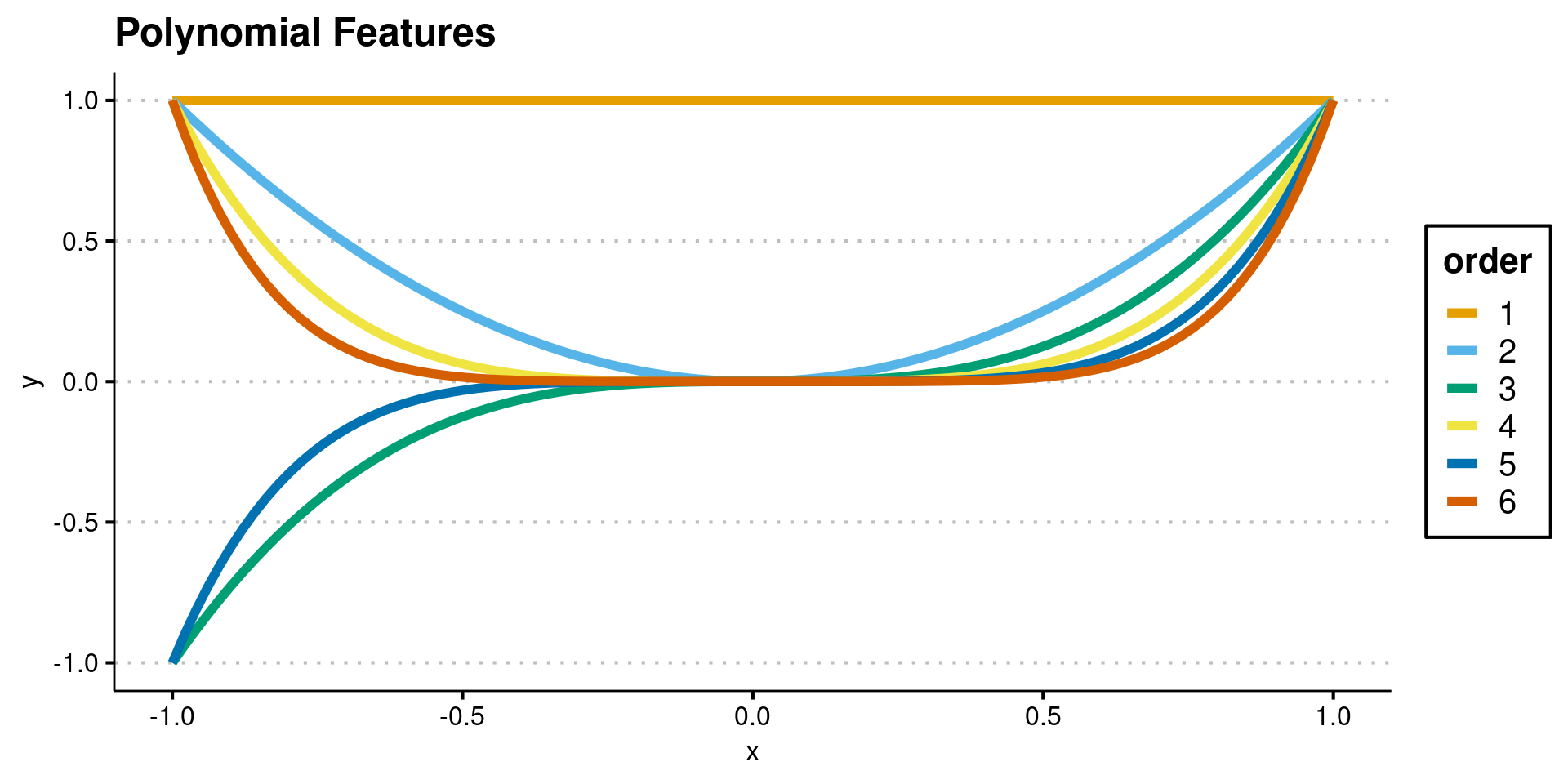
Polynomials are Bad Features

Polynomials have strong symmetries
Polynomials “blow-up” at edge of domain

Polynomials are Bad Features

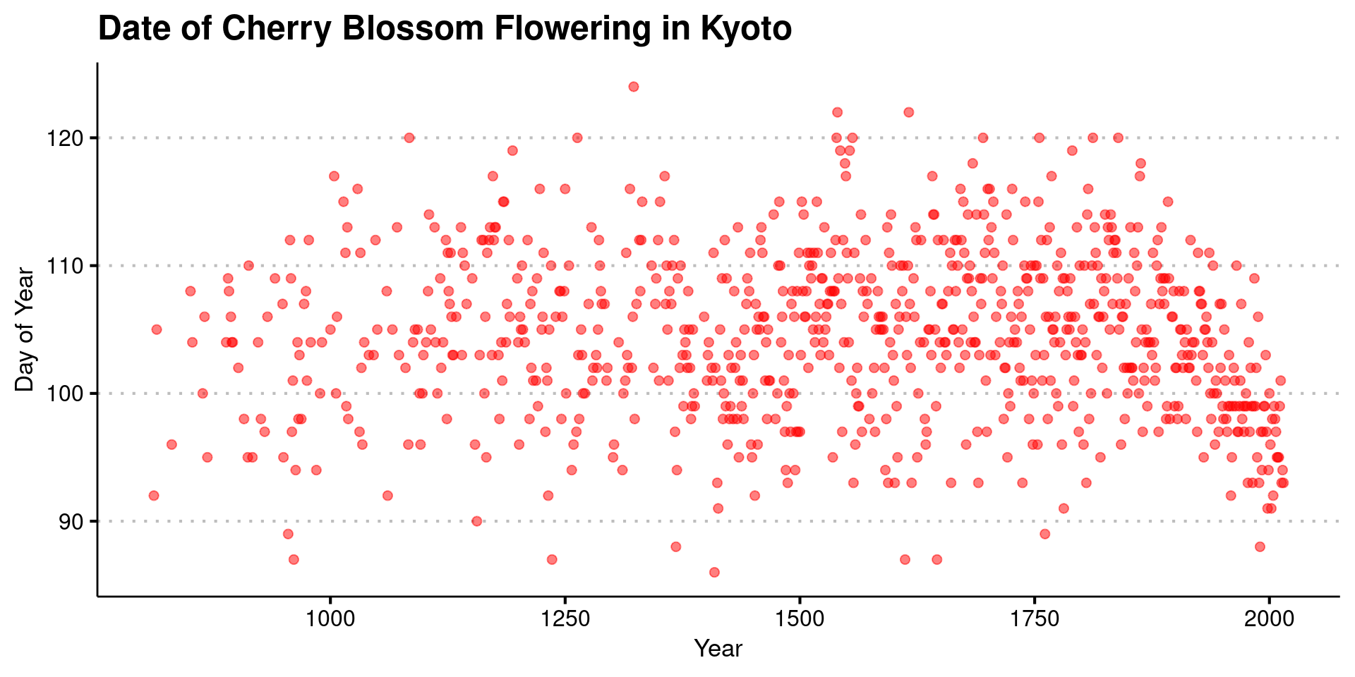
Wouldn’t it make more sense to use features with more local structure?

Example B-Splines

Idea of B-Splines is to have local features
Divide Domain into regions

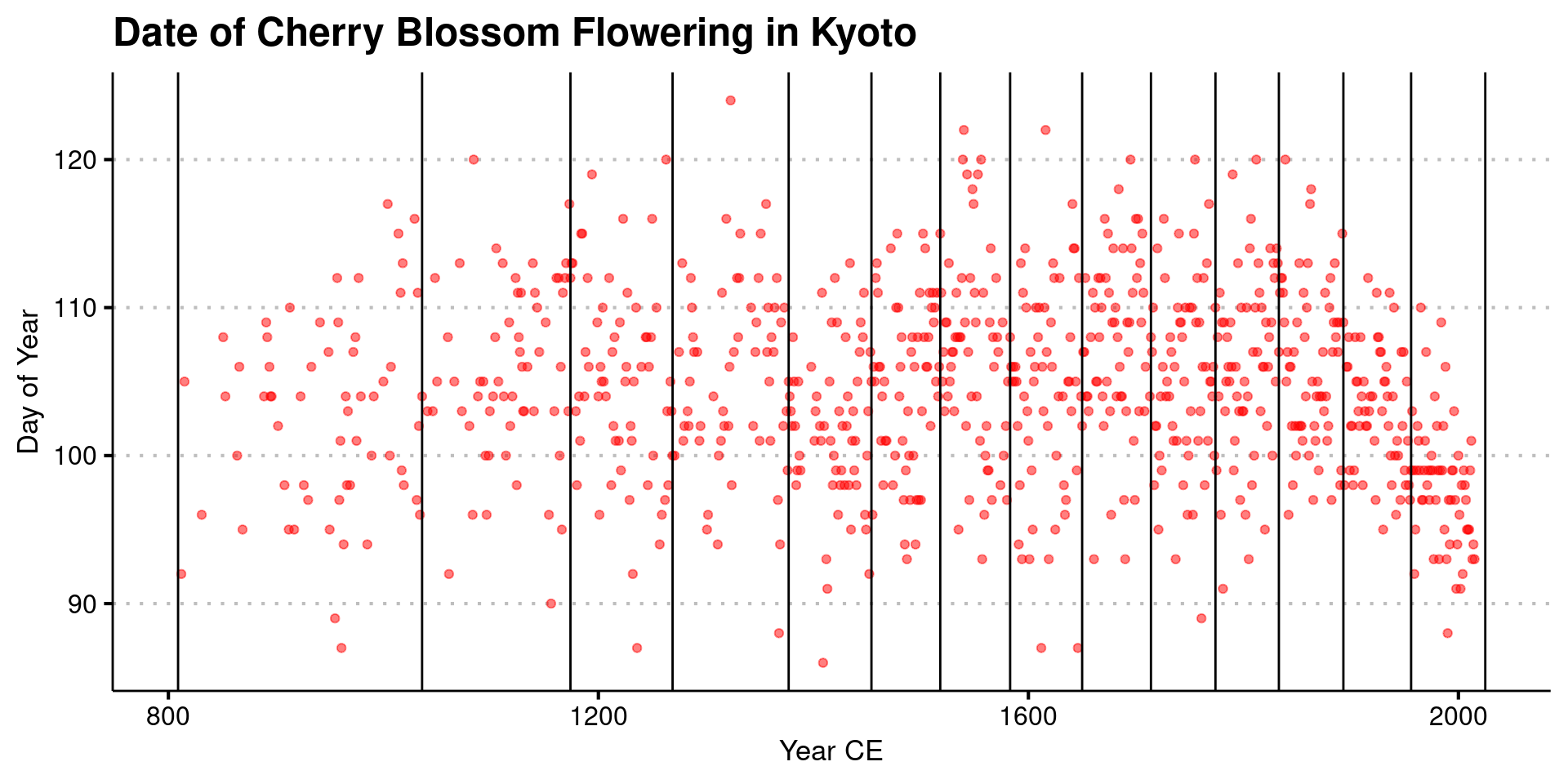
Do a fit within each region

Have a small number of basis functions within each region
Piecewise Constant: Basis is $1$

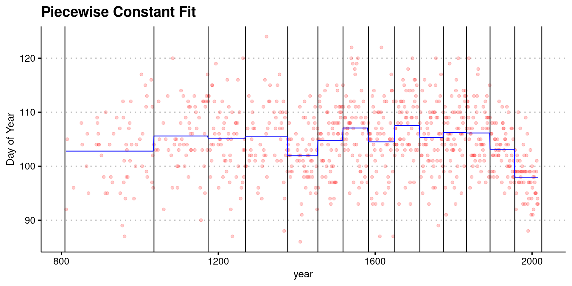
Do a fit within each region

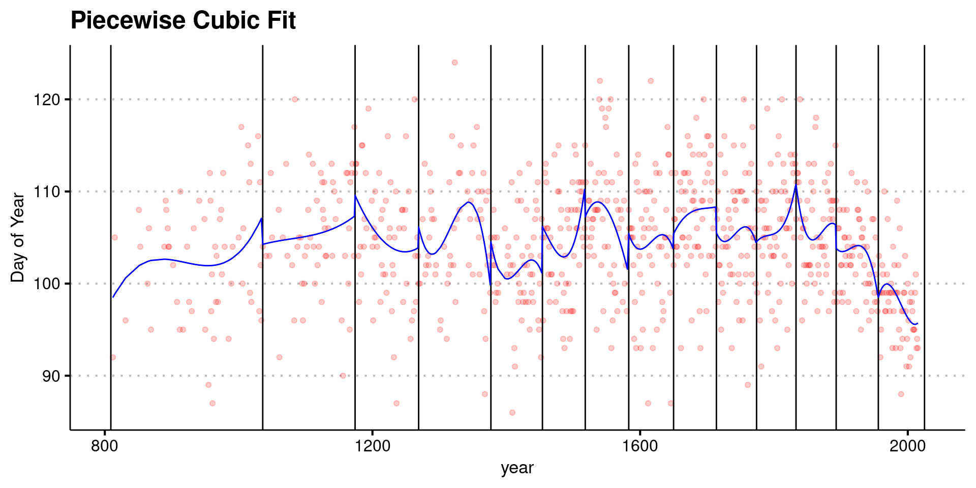
B-Spline uses more polynomials
Cubic is most common $1$, $x^2$, $x^3$, $x^4$

Piecewise Cubic Fit

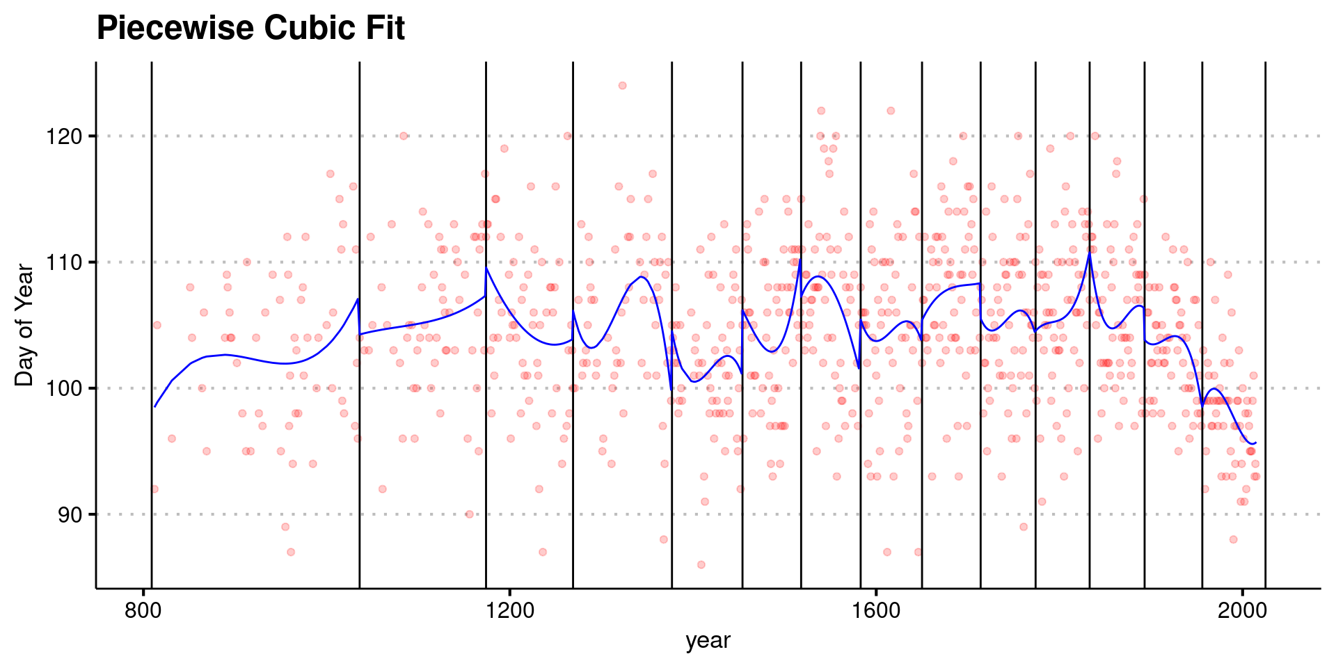
Not the jumps at each of the knots
To make the fit function “smooth” we need to add constraints

Problem that was Solved

Problem so far: \[f_{ij}(x) = x^{i-1},\quad \mathrm{if: }\quad \mathrm{knot}_j \leq x < \mathrm{knot}_{j+1},\\ f_{ij}(x) = 0,\quad \mathrm{otherwise} \]
$i \in 1\,...\,4$, $j \in 1\, ... \mathrm{number\, of\, knots}$ \[ A_{k,(4(j-1)+i)} = f_{ij}(x_k) \] \[ \min_{\theta} \|A\mathbf{\theta} - \mathbf{x}\|^2\]

Adding Constraints

Want the predictions to match at each knot: \[ \sum_{i=1}^{4} \theta_{ij}\left(\mathrm{knot}_j\right)^{i-1} = \sum_{i=1}^{4} \theta_{i,j+1}\left(\mathrm{knot_{j}}\right)^{i-1} \]
Also want derivatives to match at each knot: \[ \sum_{i=2}^{4} (i-1)\theta_{ij}\left(\mathrm{knot}_j\right)^{i-2} = \sum_{i=2}^{4} (i-1)\theta_{i,j+1}\left(\mathrm{knot_{j}}\right)^{i-2} \]

Full Problem

Each knot produces two linear equations
Can write overall as $C\mathbf{\theta} = \mathbf{d}$
Full Problem:

\[\mathrm{find:}\quad \min_{\mathbf{\theta}}\|A\mathbf{\theta} - \mathbf{x}\|^2 \\ \mathrm{subject\, to:\quad C\mathbf{\theta} = \mathbf{d}}\]

How to solve it?

Brute force way
- $C\mathbf{\theta} = \mathbf{d}$ can be solved
- Get a “hyperplane” of solutions because underdetermined
- Reformulate least squares and solve
Or use Lagrange Multipliers

Lagrange Multipliers

Constrained problem into unconstrained

\[\mathrm{find:}\quad \min_{\mathrm{\theta}} \mathbf{f}(\mathbf{\theta}) \\ \mathrm{subject\, to:} \quad \mathbf{g}(\mathbf{\theta}) = 0 \]

Lagrangian: \[ L(\mathbf{\theta},\mathbf{z}) = f(\mathbf{\theta})-\mathbf{z}^Tg(\mathbf{\theta})\]
Critical points of $L$ are potential minima of the constrained problem

Why does it work?

Critical points of $L$: \[ \frac{\partial L(\mathbf{\theta},\mathbf{z})}{\partial\theta} = \nabla \mathbf{f}(\theta) - \mathbf{z}^T\nabla \mathbf{g}(\theta) = 0 \\ \frac{\partial L(\mathbf{\theta},\mathbf{z})}{\partial\theta} = \mathbf{g}(\theta) = 0 \]
Get back the constraint equations
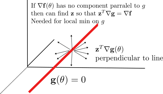
First equation says that gradient of objective has to be made parallel to gradients of constraints

Geometric Explanation

$\mathbf{g(\theta)} = 0$ defines a lower dimensional shape
- The more equations the less dimensionality of the shape
- $n$ equations gives points (0D)
- $n-1$ equations gives curves (1D)
- $n-2$ equations gives surfaces (2D)
$\mathbf{z}^T\nabla\mathbf{g}(\theta)$ is a linear combination of constraint gradients

Geometric Explanation

Lagrange Multiplier For Least Squares

\[ L(\mathbf{\theta},\mathbf{z}) = \|A\mathbf{\theta}-\mathbf{x}\|^2 + \mathbf{z}^T\left(C\mathbf{\theta}-\mathbf{d}\right) \]

Gives us:

\[ \frac{\partial L(\theta,\mathbf{z})}{\partial \theta} = 2A^T\left(A\mathbf{\theta} - \mathbf{x}\right) + C^T\mathbf{z} = 0,\\ \frac{\partial L(\theta,\mathbf{z})}{\partial \theta} = C\theta -\mathbf{d} = 0 \]

KKT Matrix

Lagrange multiplier equations are linear, can write a matrix equation: \[ \begin{bmatrix} 2A^TA & C^T \\ C & 0 \end{bmatrix} \begin{bmatrix} \mathbf{\theta} \\ \mathbf{z} \end{bmatrix} = \begin{bmatrix} 2A^T\mathbf{x} \\ \mathbf{d} \end{bmatrix} \]
Bottom row implements the constraints
Matrix is called KKT matrix

Conditions on A and C

When is KKT matrix invertible?
$n+p\times n+p$
$C$ has indepdendent
- Otherwise can’t find $\mathbf{z}$
- Implies $C$ is wide
$\begin{bmatrix} A \\ C\end{bmatrix}$ has independent columns
- Go wrong if not enough data

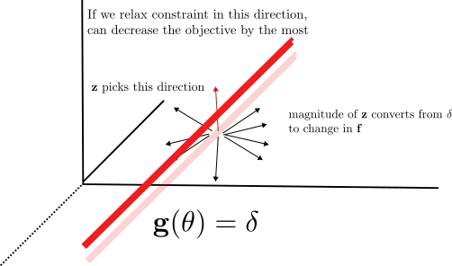
$\mathbf{z}$ are Shadow Prices

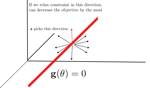
What is the meaning of the $\mathbf{z}$ from the solution?

$\mathbf{z}$ are Shadow Prices

What is the meaning of the $\mathbf{z}$ from the solution?

Shadow Prices

Let’s say your constraint is negotiable
Change your constraint to $C\theta = \mathbf{d}+\mathbf{\delta}$
Objective changes by: \[ \|A\theta_{new}-\mathbf{x}\|^2 - \|A\theta_{old} - \mathbf{x}\|^2 \approx \mathbf{z}^T\delta \]
If your objective function was a cost then $\mathbf{z}$ can be interpreted as a price per unit of constraint.

Implementing the B-Splines: Knots

num_knots = 15
knot_list <- quantile(cherry_blossoms_2$year,
                      probs = seq(from = 0, to = 1, 
                                length.out = num_knots))
regions = num_knots
num_spline = 4

cherry_blossoms_2 = cherry_blossoms_2 |> mutate(region = cut(year,breaks = knot_list,right=FALSE,labels=FALSE)) |> mutate(
  region = if_else(is.na(region),num_knots,region))

cherry_blossoms_2 = cherry_blossoms_2 |> mutate(
  adj_year = 2*(year - min(year))/(max(year)-min(year)) - 1)

normalizing the year variable is important for the condition number of resulting Gram matrix and constraints!

Implementing the B-Splines: A

A = matrix(0,nrow = nrow(cherry_blossoms_2),ncol = num_spline*(regions))

for (n in 1:nrow(cherry_blossoms_2)){
  region = cherry_blossoms_2$region[n]
  year = cherry_blossoms_2$year[n]
  adj_year = cherry_blossoms_2$adj_year[n]
  A[n,(4*(region-1) + 1):(4*(region))] = c(1,adj_year,adj_year^2,adj_year^3) 
}

For each data point, we find the corresponding region
For each region for values of theta
Calculate basis functions

Implementing the B-Spline: C

C = matrix(0,nrow = 2*(regions-1),ncol = 4*regions)

min_year = min(cherry_blossoms_2$year)
max_year = max(cherry_blossoms_2$year)

adj_knot_list = 2*(knot_list-min_year)/(max_year-min_year) - 1

for (i in 1:(regions-1)){
  C[2*i-1,(4*(i-1)+1):(4*i+4) ] = c(1,adj_knot_list[i+1],
      adj_knot_list[i+1]^2, adj_knot_list[i+1]^3,
  -1, -adj_knot_list[i+1], -adj_knot_list[i+1]^2,
  -adj_knot_list[i+1]^3)

    C[2*i,(4*(i-1)+1):(4*i+4)] = c(0,1,2*adj_knot_list[i+1],
    3*adj_knot_list[i+1]^2, 0, -1, -2*adj_knot_list[i+1],
    -3*adj_knot_list[i+1]^2)
}

Forming the KKT Matrix and RHS

n_thetas = ncol(A)
p_constraints = nrow(C)
KKT = matrix(0,nrow = n_thetas+p_constraints ,n_thetas+p_constraints)

KKT[1:n_thetas,1:n_thetas] = 2*t(A) %*% A
KKT[1:n_thetas,(n_thetas+1):(n_thetas+p_constraints)] = t(C)
KKT[(n_thetas+1):(n_thetas+p_constraints),1:n_thetas] = C

rhs_ext = matrix(0,nrow = n_thetas+p_constraints,ncol = 1)

doy = cherry_blossoms_2$doy

rhs_ext[1:n_thetas,1] = 2*t(A) %*% doy

Solving the Problem

theta_ext = solve(KKT,rhs_ext)
theta_sol = theta_ext[1:n_thetas]
z_sol = theta_ext[(n_thetas+1):(n_thetas+p_constraints)]

doy_pred = A %*% theta_sol

cherry_blossoms_2 |> mutate(doy_pred = doy_pred) |> 
  ggplot(aes(x=year,y=doy)) + geom_point(color="red",alpha=0.2) +
  geom_vline(data = knot_df,mapping = aes(xintercept=knots)) +
  geom_line(mapping = aes(x= year, y = doy_pred), color = "blue") +
    labs(title="B-Spline Fit") +
    ylab("Day of Year") +
  theme_clean(base_size = 16)

Solving the Problem

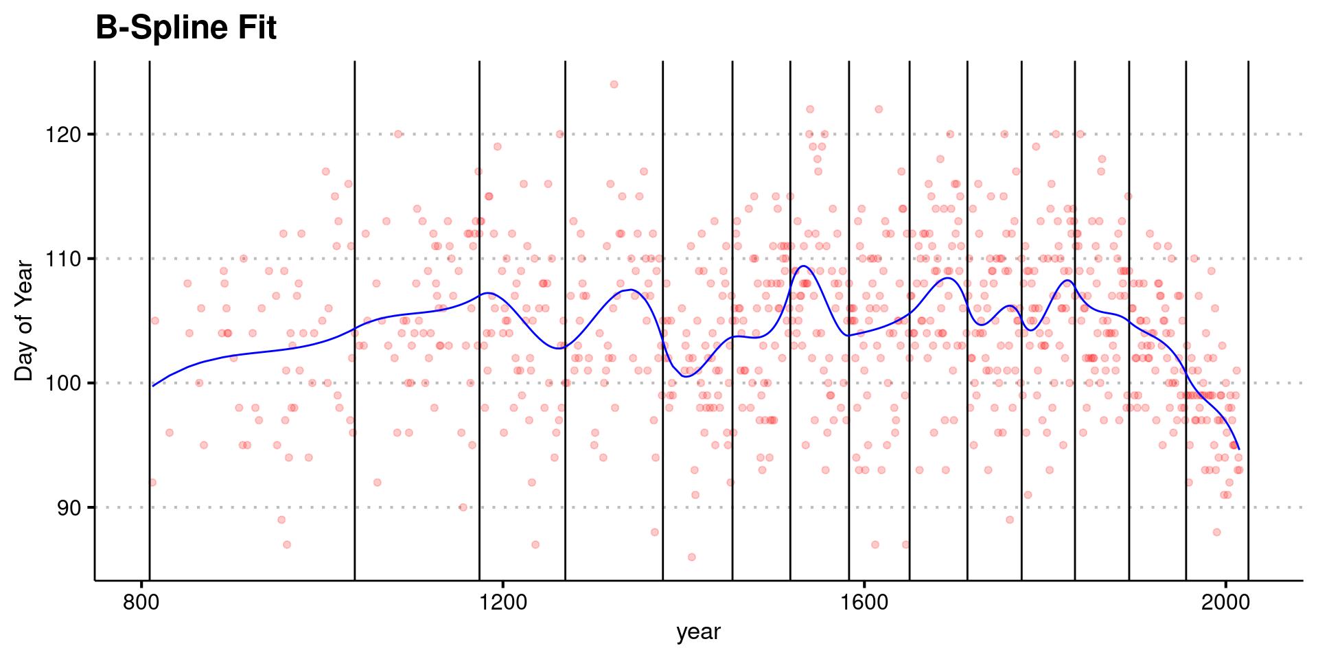
Jumps are gone!

Example: Portfolio Optimization

You have a budget of $d$ dollars to invest in financial assets
Portfolio allocation weights $\mathbf{w}$ describe how much you invest in each asset
You will hold the portfolio over some well defined period

Portfolio Terminology

Short positions, $w_i < 0$ for some $i$
Leverage = $\sum_{i=1}^n |w_i|$
- Measures how much money you have borrowed
- Have to pay interest in real world
Risk Free Asset
- Usually one asset is a cash or treasury equivalent with low to no risk and return

Portfolio Returns

On day $t$, value of asset $i$ changes by $R_{it}$
$R_{it} = 1.05$ is a $5\%$ gain, $0.91$ a $9\%$ loss, $0$ a 100% loss, etc
After an investment period of $T$ days, overall portfolio value: \[ d_T = d\sum_{i=1}^n\Pi_{t=1}^T R_{it}w_i \]
Note that returns are multiplicative over time
Often annualize return: $\rho_{A} = \rho_T^{T_y/T}$, where $T_y$ trading days per year

Portfolio Risk

Day to day variability of portfolio is called risk
Define $\bar{\rho} = \frac{1}{T}\sum_{t=1}^T \sum_{i=1}^n R_{it}w_t$
Compute variance \[ \mathrm{var}\left(\rho\right) = \frac{1}{T}\sum_{t=1}^T\left(\sum_{i=1}^n R_{it}w_i - \bar\rho \right)^2 \]
Annualized risk defined as $\sqrt{T_{y}}\sqrt{\mathrm{var(\rho)}}$

Covariance Formulation

Can also measure risk based on covariance matrix between daily returns of each asset: \[ \Gamma_{ij} = \frac{1}{T}\sum_{i=1}^T \left(R_{it} -\bar{\rho}_i\right)\left(R_{jt} - \bar{\rho}_j\right) \]
Then: \[ \mathrm{var}(\rho) = \mathbf{w}^T\Gamma\mathbf{w} \]

Markowitz Portfolio Optimization

Goal: Use past data to estimate future returns $\rho_i$ and correlations $\Gamma$
Calculate portfolio weights $\mathbf{w}$ to minimize risk while achieving a target return

\[ \mathrm{find:}\quad \min_{\mathbf{w}} \mathbf{w}^T\Gamma\mathbf{w} \\ \mathrm{subject\, to:}\quad \sum_{i=1}^n w_i = 1 \\ \sum_{i=1}^n \rho_i w_i = \rho_{g} \]

This is a least squares (actually least norm) problem with $\Gamma$ taking role of Gram matrix $A^TA$

Risk Return Tradeoff

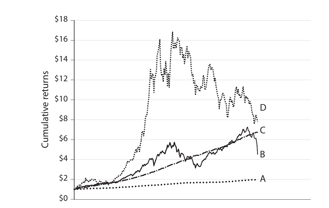
Which asset would you pick?

Andrew Lo AM

Risk Return Tradeoff

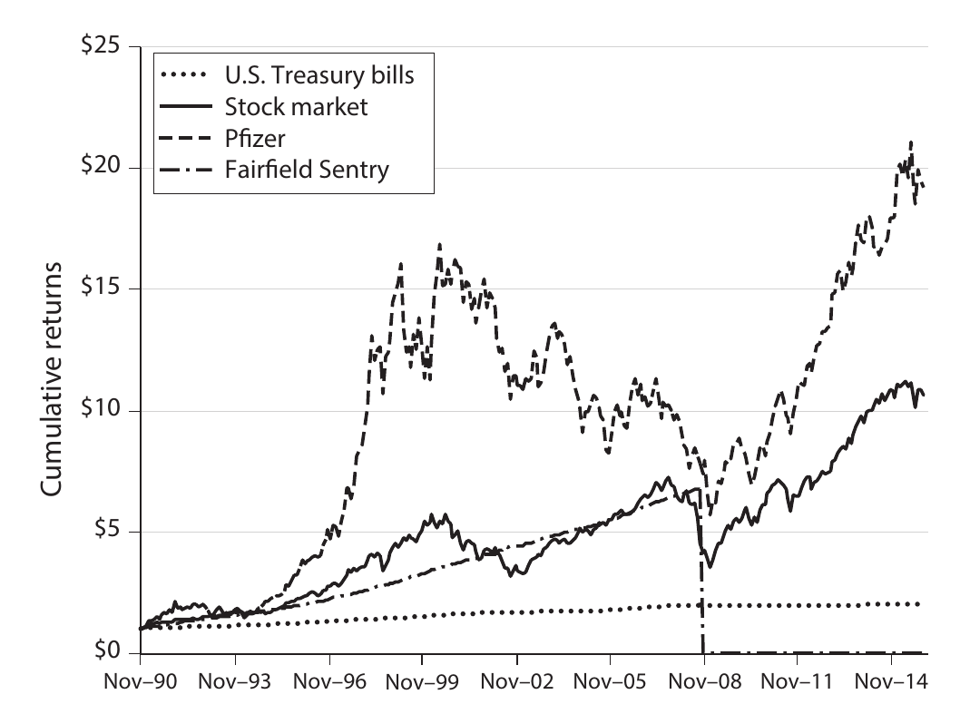
Medium reward “no risk” asset was Bernie Madoff

Andrew Lo AM

Risk Return Tradeoff

Minimizing risk at a high return target leads to high leverage
Risk to go bust out of sample

Meetup 4: Constrained Least Squares

Everything in life has constraints

Everything in life has constraints

Everything in life has constraints

Everything in life has constraints

Weekly Summary

Events Happening this Week!

Events Happening this Week

Events Happening This Week!

Events Happening this Week

Constrained Least Squares

Alternative Formulation

Why Just Equality?

Example: B-Splines

Polynomials are Bad Features

Polynomials are Bad Features

Example B-Splines

Do a fit within each region

Do a fit within each region

Piecewise Cubic Fit

Problem that was Solved

Adding Constraints

Full Problem

How to solve it?

Lagrange Multipliers

Why does it work?

Geometric Explanation

Geometric Explanation

Lagrange Multiplier For Least Squares

KKT Matrix

Conditions on A and C

\(\mathbf{z}\) are Shadow Prices

\(\mathbf{z}\) are Shadow Prices

Shadow Prices

Implementing the B-Splines: Knots

Implementing the B-Splines: A

Implementing the B-Spline: C

Forming the KKT Matrix and RHS

Solving the Problem

Solving the Problem

Example: Portfolio Optimization

Portfolio Terminology

Portfolio Returns

Portfolio Risk

Covariance Formulation

Markowitz Portfolio Optimization

Risk Return Tradeoff

Risk Return Tradeoff

Risk Return Tradeoff

Thanks!