DATA 609 Meetup 10: Applications to Data Fitting
George I. Hagstrom
Week Summary
- Starting a two week block on applications to stats/ML
- Chapter 6, 7 of
cvxbook
- Chapter 6, 7 of
- Finish off convex optimization with duality
- Lab 5 due this Sunday at midnight
Norm Approximation
- Find coefficients \(\mathbf{x}\) that minimize: \(\|A\mathbf{x}-\mathbf{b}\|\)
- Here \(\|\cdot\|\) is any norm
- Can have convex constraints on \(\mathbf{x}\)
A norm is a mathematical measure of distance
- Several ways to do it, share key properties
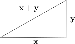
- Shortest distance is straight line (triangle inequality): \[ \|\mathbf{x} + \mathbf{y}\| \leq \|x\| + \|y\| \]
A norm is a mathematical measure of distance
- Several ways to do it, share key properties
- Shortest distance is straight line (triangle inequality): \[ \|\mathbf{x} + \mathbf{y}\| \leq \|x\| + \|y\| \]
- Positive \(\|\mathbf{x}\|\geq 0\)
- Homogeneous \(\|s\mathbf{x}\| = |s|\|\mathbf{x}\|\)
- Norms are convex
Important Norms
- Euclidean or 2-Norm: \(\|\mathbf{x}\|_2 = \left(\sum_i x_i^2\right)^{1/2}\)
- \(L_1\) Norm: $||_1 = _i |x_i|
- \(L_{\infty}\) Norm: \(\|\mathbf{x}\|_{\infty} = \mathrm{\max}_i \{x_i\}\)
Level Sets of Norms
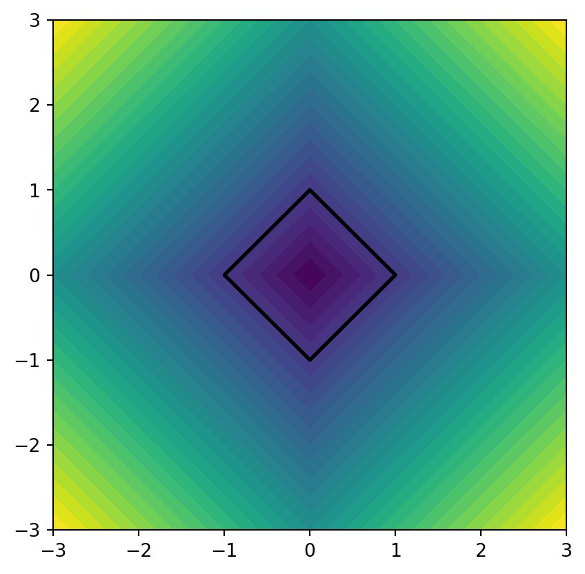
- \(L_1\) norm sometimes called taxicab distance
- Dark Lines on Axes cause sparsity in applications
Level Sets of Norms
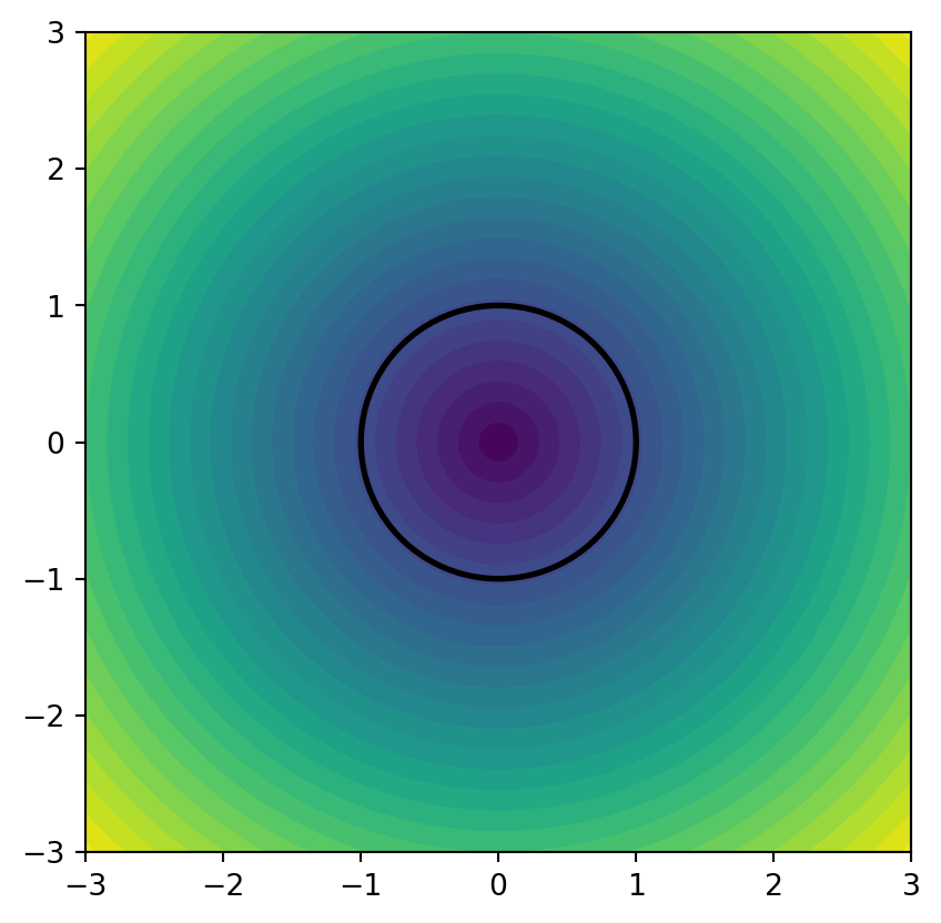
- Euclidean Distance
- Least Squares
Level Sets of Norms
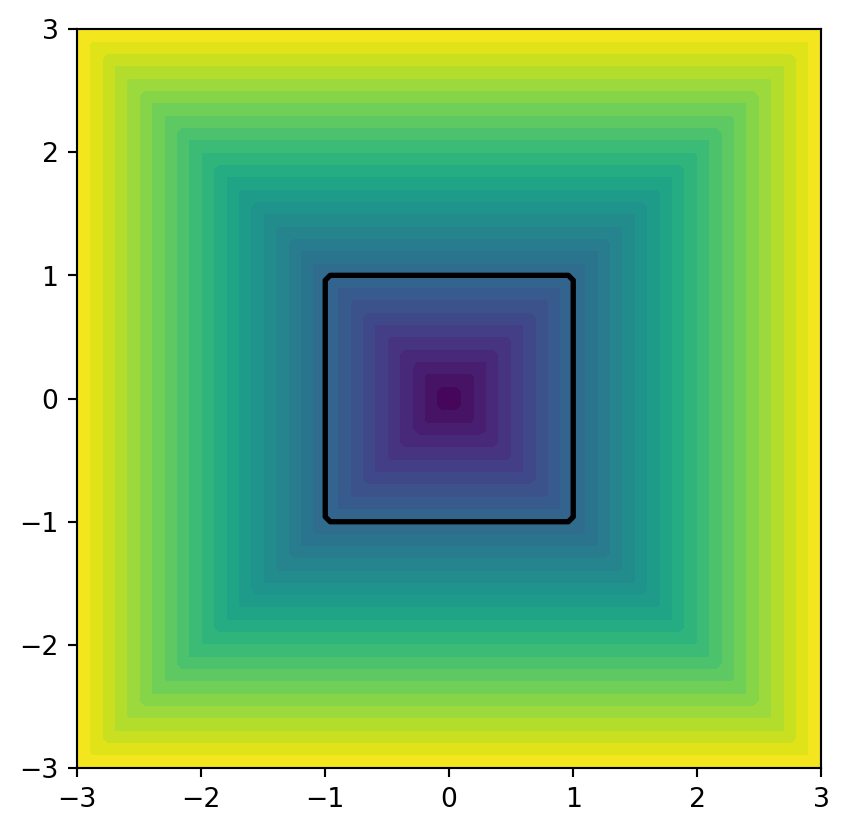
- \(L_{\infty}\) measures maximum element
Penalty Functions
- Can generalize this further to sum of convex penalty functions \[ \min_{x} \sum_{i} \phi\left((A\mathbf{x}-b)_i\right) \]
- penalty function \(\phi \geq 0\)
- \(\phi(0)=0\)
- \(\phi\) increasing for argument larger than \(0\), decreasing when it is smaller than \(0\)
Important Penalty Functions
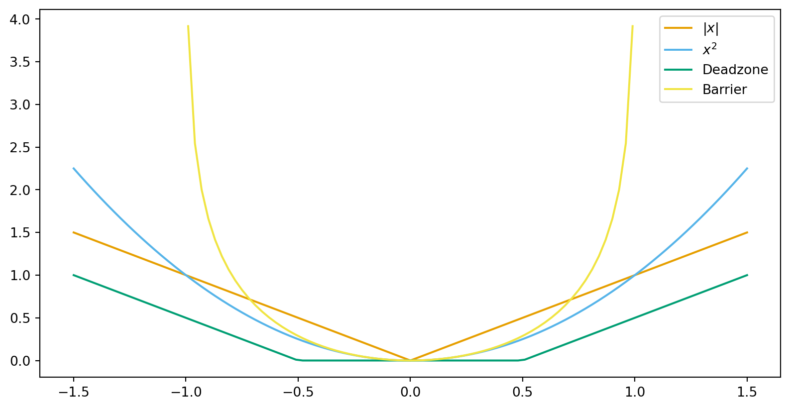
- \(\phi(x) = |x|\), \(\phi(x) = x^2\) lead to norm problems
- \(\phi(x) = \mathrm{\max}\{0,|x|-a\}\) dead-zone linear
- If you are close enough no penalty, otherwise linear
- \(\phi(x) = -\log(1-x^2)\),
log-barrierpenalty- Blows up at \(x=\pm 1\)
Visualizing Penalties
Robustness to Outliers
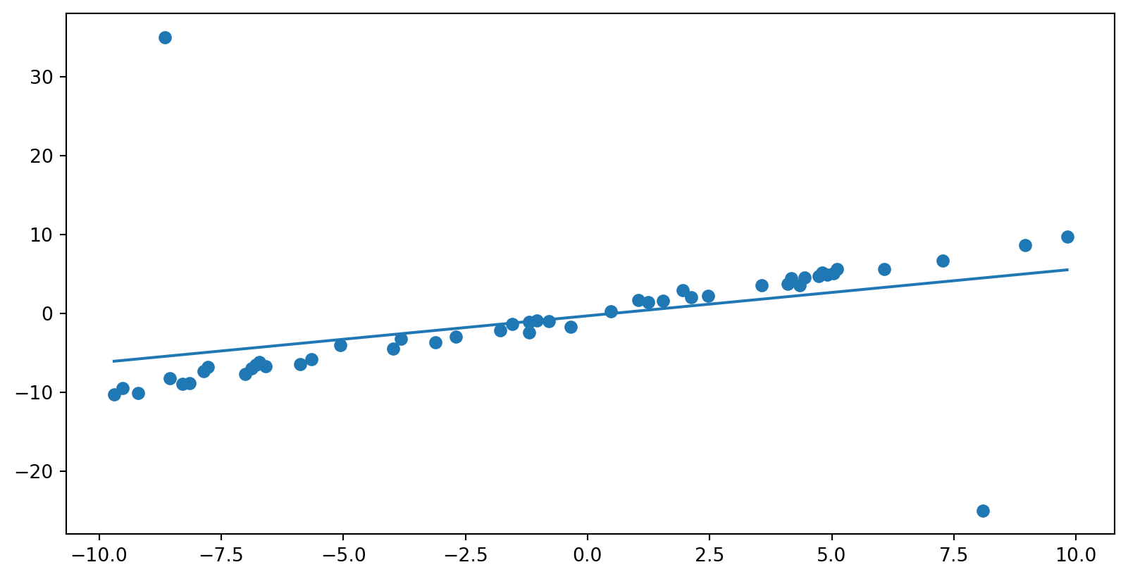
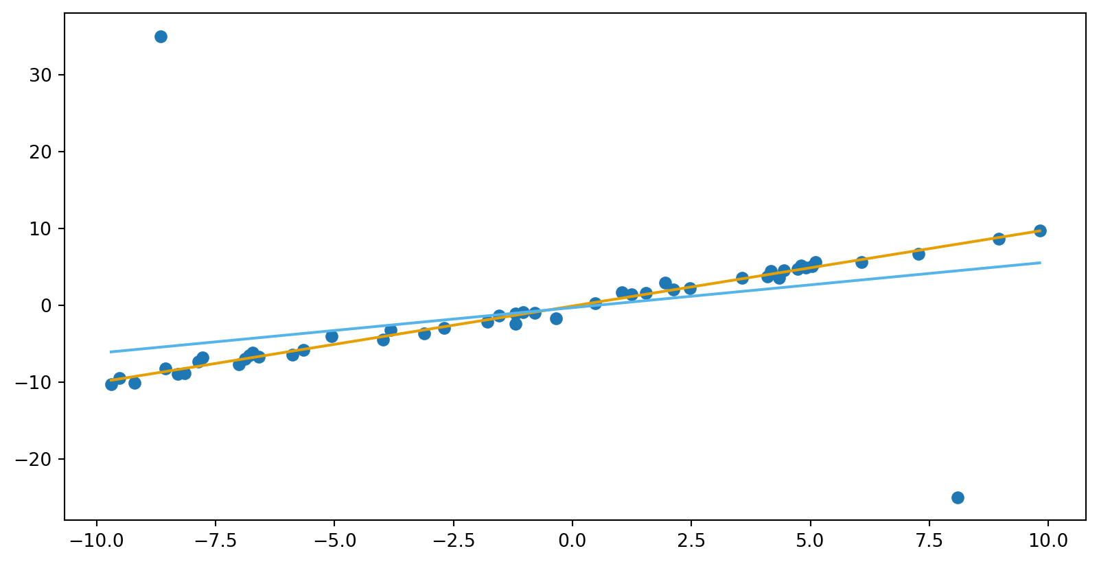
- An outlier is a data point that was generated by a different process than the other points in the dataset
- Could be due to an interesting phenomenon
- Could be due to a mistake, in which case it is called a spurious value
- Problem: Stats based on Gaussian Distribution (and thus quadratic penalty) are not robust to outliers
Linear Regression Examples
Robust Regression
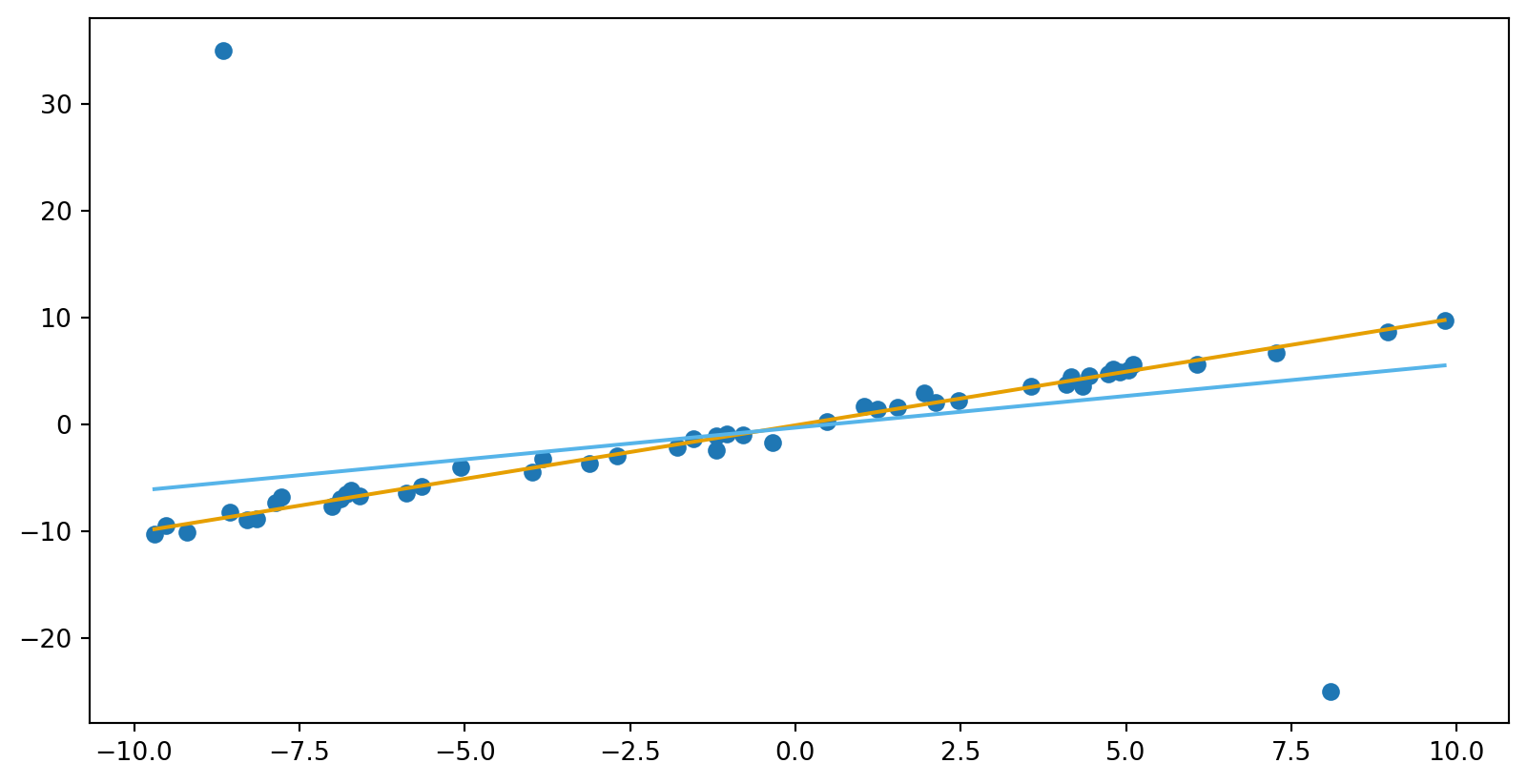
- Quadratic penalty squares residuals
- Penalizes large errors much more than small ones
- Absolute value penalizes residuals equally, so less sensitive to outliers
- Robust Regression is \(L_1\) penalized linear regression
Robust Regression
Huber Penalty
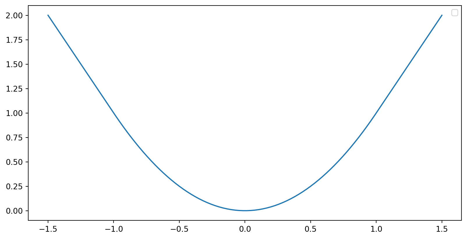
- Quadratic penalty is optimal when we have Gaussian errors
- Huber function is a compromise between quadratic and absolute value: \[ \phi_h(x) = \begin{cases} x^2 & \mathrm{if}\quad |x|< M \\ M\left(2|x|-M\right) & \mathrm{if}\quad |x|\geq M \end{cases} \]
Huber Penalty
Huber Regression
- Huber Penalty also leads to robust fits
- Should pick \(M\) based on a robust estimate of the standard deviation \(\sigma\)
- Want the quadratic part to be in force when errors produced by Gauassian
- Want linear part for larger errors
Huber Regression
Least Norm Problems
\[ \mathrm{min} \|\mathbf{x}\| \\ A\mathbf{x} - \mathbf{b} = 0 \]
- Equivalent to norm approximation
- System is underdetermined
- \(\mathbf{x} = \mathbf{x}_0 + Z\mathbf{u}\)
- \(\mathrm{min}_{\mathbf{u}}\|\mathbf{x}_0 + Z\mathbf{u}\|\)
Regularization and Sparsity
- Least Norm lets you “solve” underdetermined linear systems
- We have also discussed regularization: \[ \mathrm{min}_{\mathbf{x}} \|f(\mathbf{x})\| + \lambda\|\mathbf{x}\| \]
- What are the trade-offs between different penalties?
\(L_1\) induces sparsity and bias
- Big difference between quadratic and abs penalty when coefficients are small:
- \(|x| \gg x^2\)
- Lasso induces sparsity- actually zeros out coefficients with small effect
- Sparsity can give big computational efficiency advantage and improve interpretability
- Can lead to bias (inaccuracy)
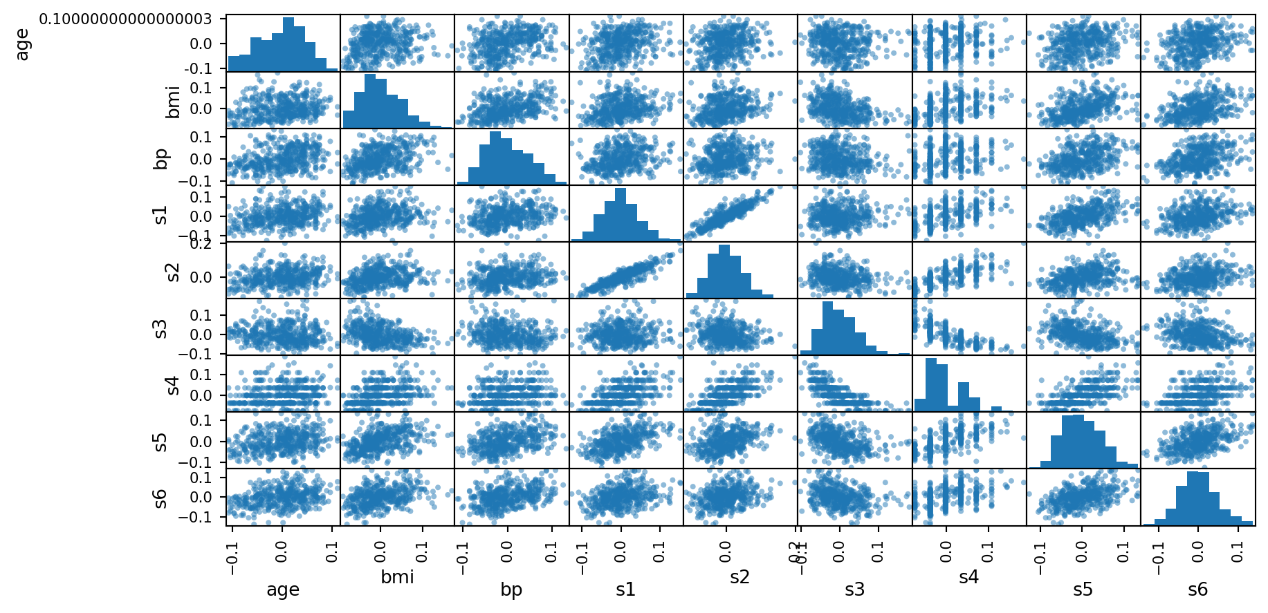
Comparison On Diabetes Dataset
- Predictor variables: age, sex, bmi, bp, and six blood test values taken at baseline
- Target variable: Measure of diabetes progression one year later
Comparisons on Diabetes Dataset
Ridge Regression
Ridge Regression
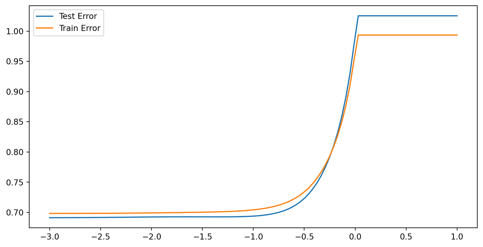
- In ridge regression the coefficients shrink together
Text(0.5, 0, 'log(lambda)')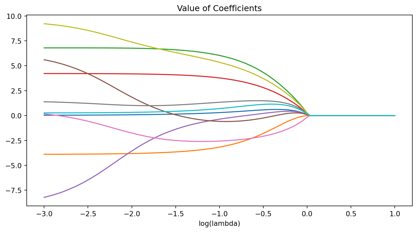
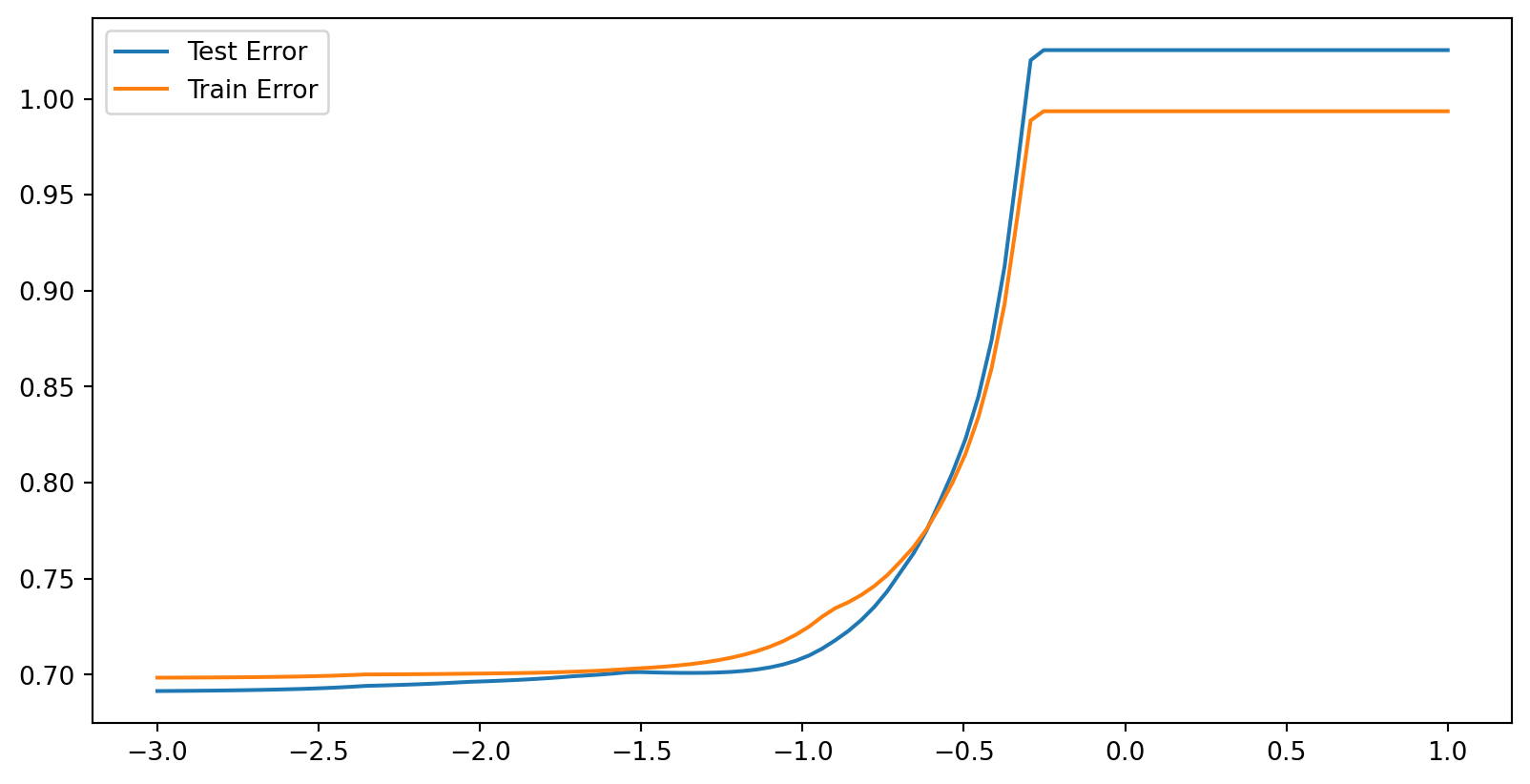
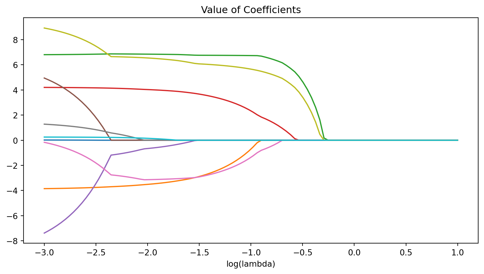
Lasso Regression
Lasso Regression
- Coefficients forced to 0 one at a time
Stochastic Robust Approximation
- Start off with a problem where we are minimizing a convex objective
- Could be least squares type like the one we write below, but doesn’t have to be: \[ \mathrm{min}_x\|A\mathbf{x}-\mathbf{b}\| \]
- Suppose that \(A\) and \(\mathbf{b}\) are actually uncertain
- Could correspond to things like measurement error
Stochastic Robust Approximation
- Reformulate problem, minimize expected value of objective: \[ \min_{x}\int dA d\mathbf{b}\left( p(A,\mathbf{b})\|A\mathbf{x}-\mathbf{b}\| \right) \]
- This is convex, but viciously hard
- Generally will have to approximate the integral
- Equivalent to discretizing distribution
Discrete Version
- Consider Discrete Version \[ \mathrm{min}_{\mathbf{x}} \sum_{i}\sum_j p_{ij}\|A_i\mathbf{x}-\mathbf{b}_j\| \]
- Could be a lot of terms but is convex
Worst Case Robust Optimization
- Idea: Instead of minimizing expected value, minimize worst case error \[ \mathrm{min}_{\mathbf{x}} \mathrm{sup}_{A} \|A\mathbf{x}-\mathbf{b}\| \]
- Convex, but still can be viciously hard
Problem 3 on Homework
- Start with logistic regression: \[ l(\theta) = \sum_{i=1}^n \log\left(1 + \exp\left(-y_i\theta^T\mathbf{x}_i\right)\right) \]
- \(y_i = \pm 1\)
- \(\theta\) coefficients
- \(\mathbf{x}_i\) is \(i\)th data point
Problem 3 Tips
- Now we assume that each \(\mathbf{x}_i\) has an error \(\delta_i\) which has maximal element of \(\epsilon\)
- New Convex Optimization Problem:
\[ l_{wc}(\theta) = \sum_{i=1}^n \sup_{\|\delta_i\|_{\infty}\leq\epsilon}\log\left(1+\exp\left(-y_i\theta^T\left(\mathbf{x}_i+\delta_i\right)\right)\right) \]
How to deal with this?
\[ l_{wc}(\theta) = \sum_{i=1}^n \sup_{\|\delta_i\|_{\infty}\leq\epsilon}\log\left(1+\exp\left(-y_i\theta^T\left(\mathbf{x}_i+\delta_i\right)\right)\right) \]