DATA 609 Meetup 13: Optimization Algorithms

George I. Hagstrom

Week Summary

  • Final Lab is Almost Ready
    • It took lots of programming to prep it
  • This week: Algos
  • Next Week: Neural Nets
  • Last Week: Deep Nets

Reading

Meetup May 7th!

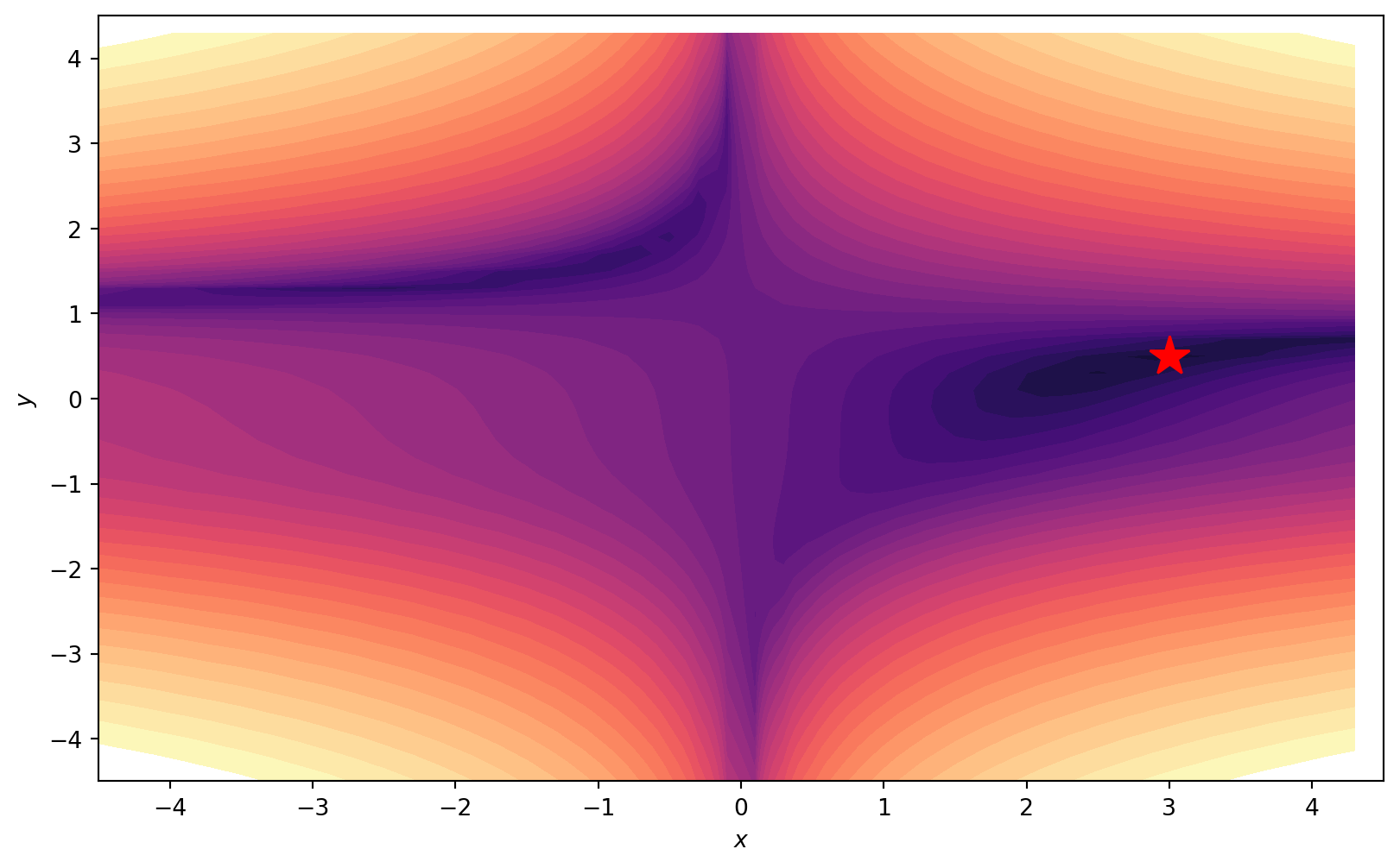
Non-Convex Optimization
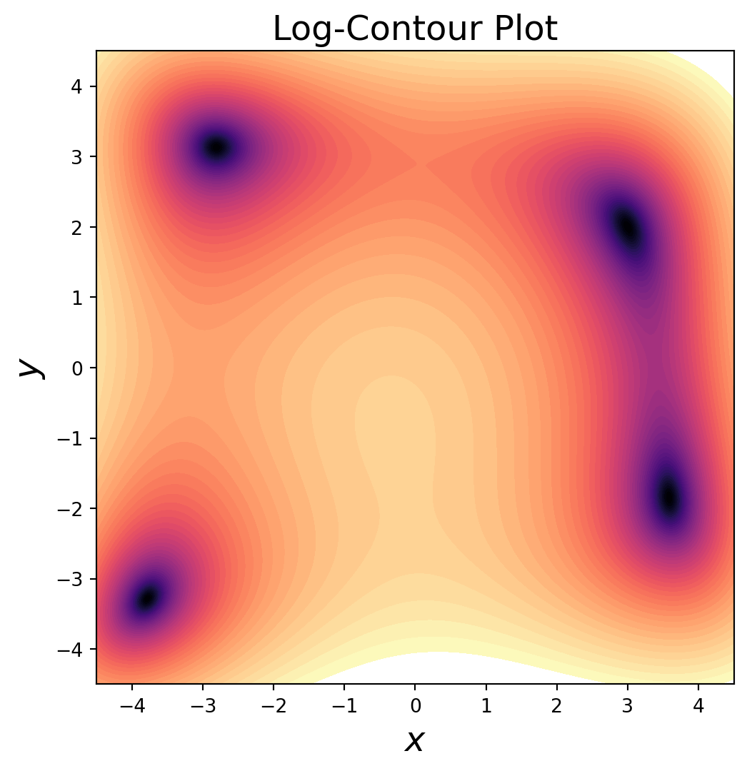
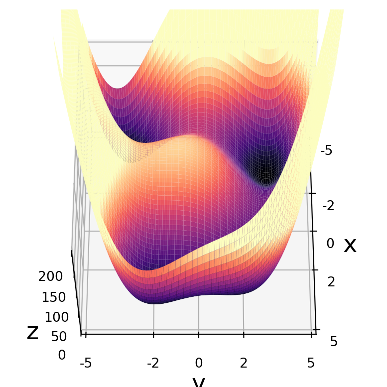
  • Can’t guarantee global minimum
  • Can find local minima
  • Heuristics over theory

Non-Convex Optimization

  • Can’t guarantee global minimum
  • Can find local minima
  • Heuristics over theory

Revisiting Gradient Descent

  • Simplest algorithm for finding a minimum
  • Start with initial guess \(\mathbf{x}_0\)
  • Compute the gradient \(\nabla f(\mathbf{x}_0)\)
  • Gradient tells us slope of landscape
  • Take steps down slope: \[ \mathbf{x}_i = \mathbf{x}_{i-1} -\kappa\nabla f(\mathbf{x}_{i-1}) \]

GD Limited by Condition Number

  • Learning rate stability constraint: \(\kappa < \frac{\lambda_{\mathrm{max}}}{\lambda_{\mathrm{min}}} = c\)
    • Pretending we are closing in on a minimum
    • Convergence Rate limited by step size: \[ \|\mathbf{x}_{\mathrm{opt}}-\mathbf{x}_i\| \sim \left(1-\frac{\lambda_{\mathrm{min}}}{\lambda_{\mathrm{max}}}\right)^{i} \]

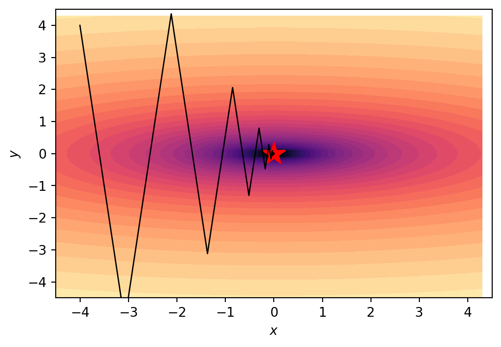
Valley Oscillation

  • High Condition number indicates narrow, steep valley
  • GD trajectories bounce up steep valley slopes
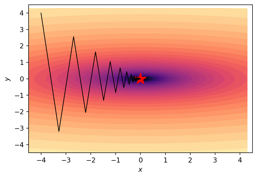
  • \(f(x,y) = x^2 + 10y^2\)
  • \(\kappa = 0.09\)

Gradient Descent with Momentum

  • Imagine rolling a ball in a channel with steep sides
  • Friction reduces movement up sides
  • Builds momentum rolling down channel

Gradient Descent with Momentum

  • Introduce “velocity” variable \[ \mathbf{x}_{i+1} = \mathbf{x}_i - \mathbf{v}_i \]
  • Gradient drives velocity, momentum provides memory:

\[ \mathbf{v}_{i+1} = \kappa\nabla f(\mathbf{x})_i + \beta \mathbf{v}_i \]

  • Oscillations damp due to memory

GD with Momentum

def gd_with_mom(grad, init, n_epochs=5000, eta=10**-4, beta=0.9,gamma=0.9):
    params=np.array(init) # Start with initial condition
    param_traj=np.zeros([n_epochs+1,2]) # Save the entire trajecotry
    param_traj[0,]=init # Also save the initial condition to the trajectory
    
    v=0 # Starting with 0 momentum
    
    # Epochs is borrowing term from machine learning
    # Here it means timestep
    
    for j in range(n_epochs): 
        v=gamma*v+(np.array(grad(params))) # Compute v
        params=params-eta*v  # Update the location
        param_traj[j+1,]=params # Save the trajectory
    return param_traj

GD with Momentum

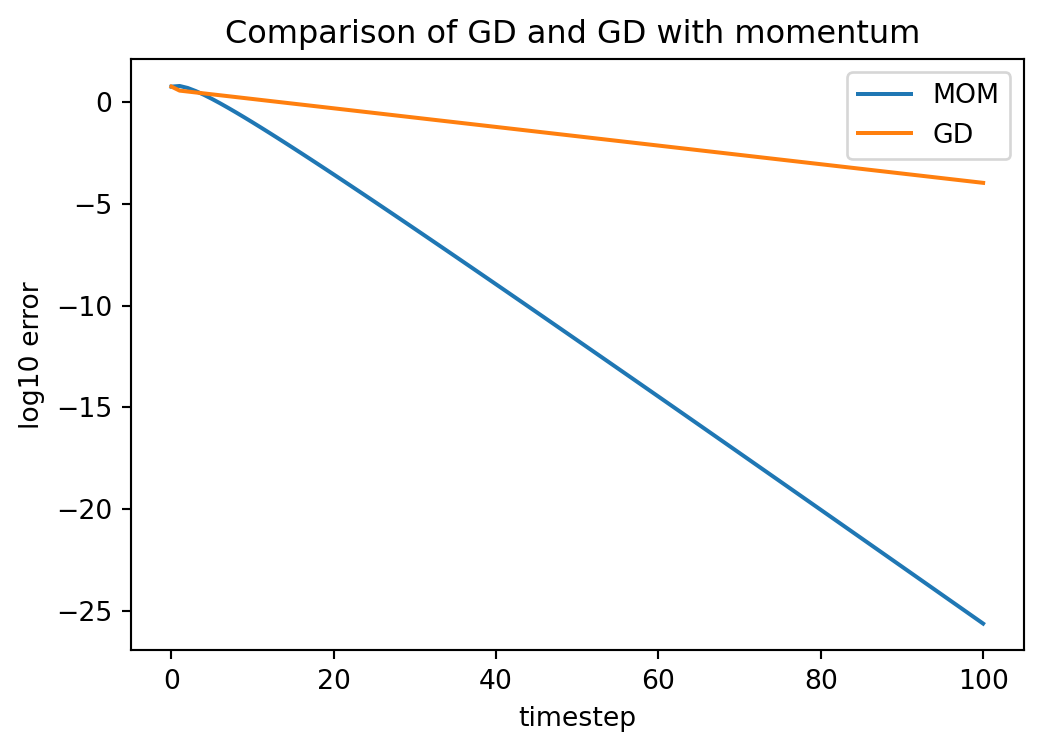
  • Momentum steps move horizontally more
  • Momentum error dramatically better

Hyperparameters?

  • Both cases I picked parameters close to optimal
  • See analysis in Strang
  • \(\kappa = 0.05\) for GD
  • \(\kappa = \left(\frac{2}{\sqrt{\lambda_{\mathrm{min}}}+\sqrt{\lambda_{\mathrm{max}}}}\right)^2\), and \(\beta = \left(\frac{1-c^{-1/2}}{1+c^{-1/2}}\right)^2\) for GD with momentum
  • Error gap increases as \(c\) increases

Hyperparameters

  • But we don’t know \(c\) in advance, varies locally….
  • We handle this several ways:
    • Experimentation
    • Heuristics
    • Adaptive Methods

Stochastic Gradient Descent

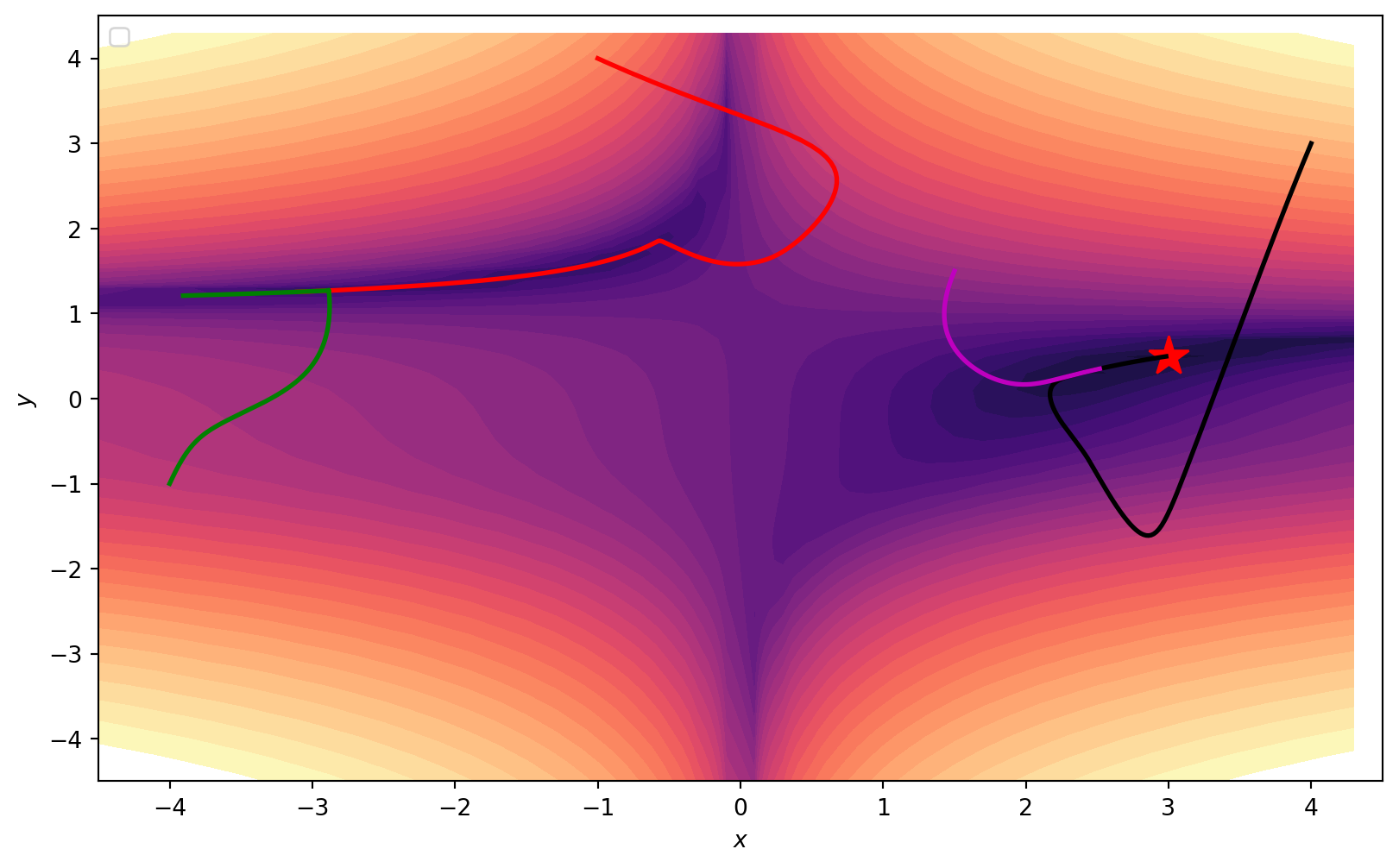
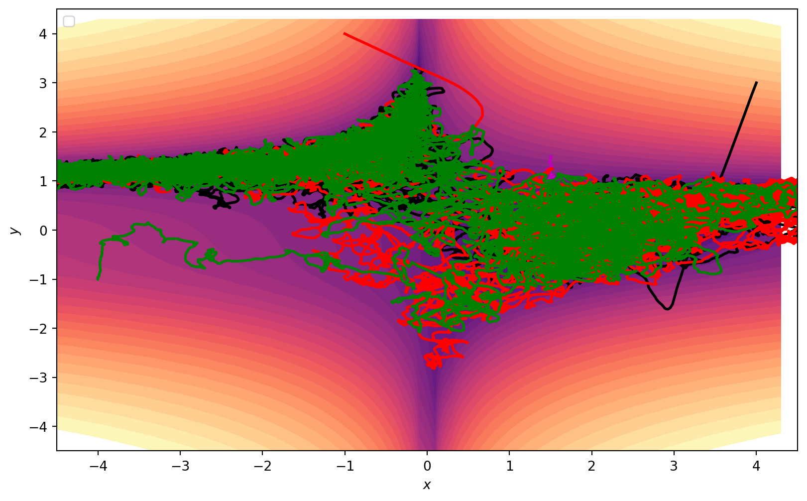
  • Common for optimization algorithms to “get stuck”
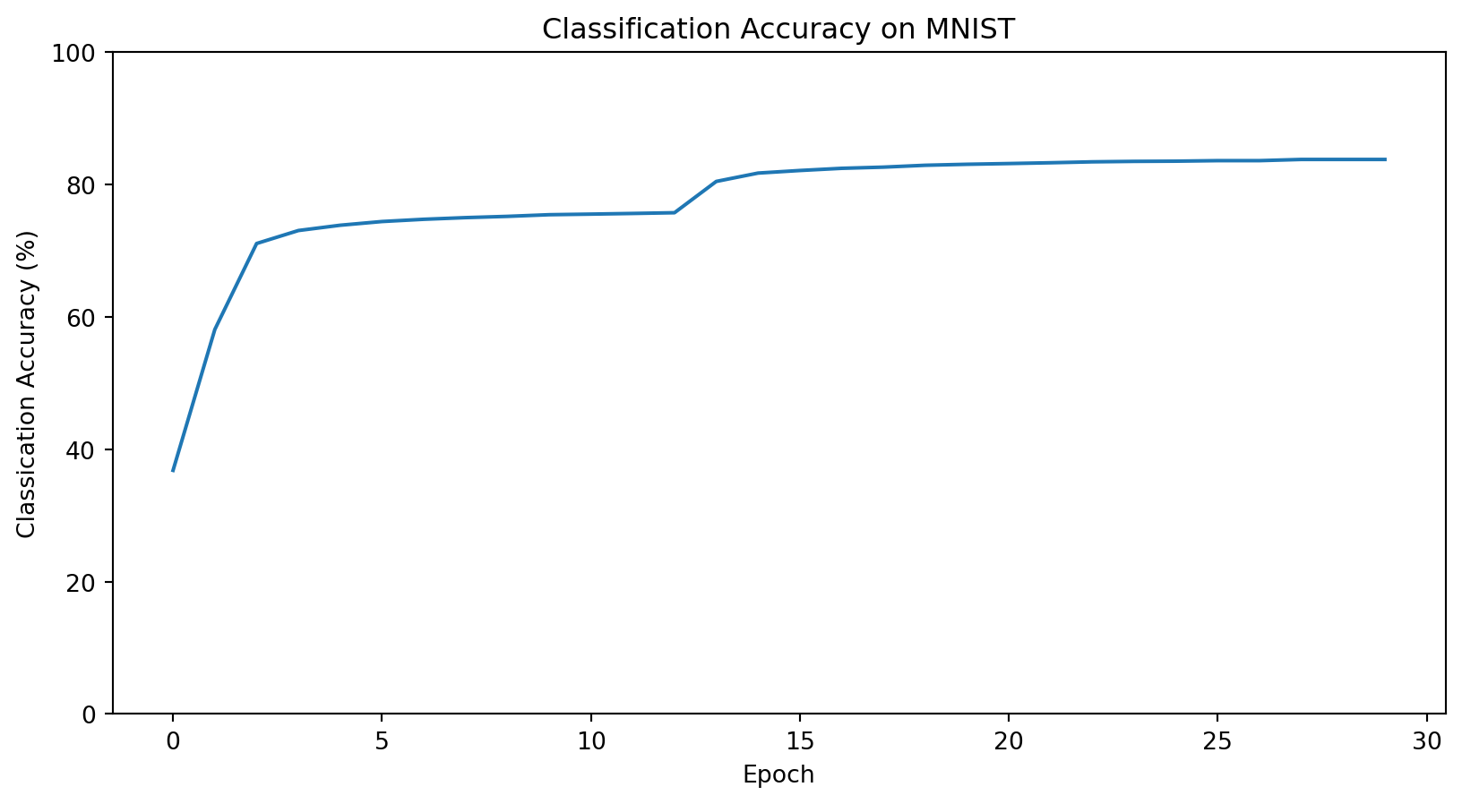
Stochastic Gradient Descent

  • In low-D local minima are problematic

Stochastic Gradient Descent

  • Trajectories get Stuck

Stochastic Gradient Descent
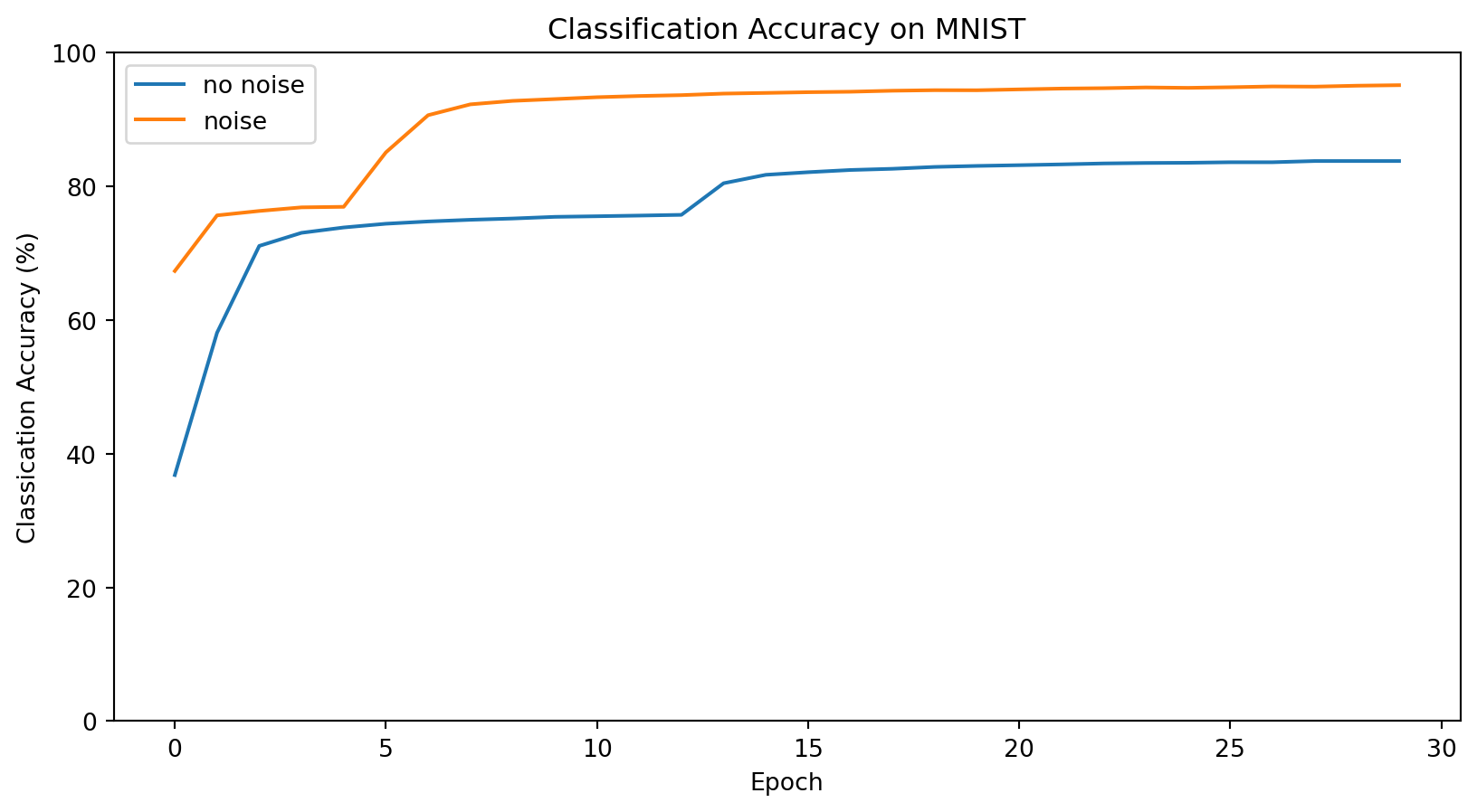
  • The barriers in high dimensions likely more complex
  • Stochastic Gradient Descent modifies gradient descent style methods
    • Compute the gradient of loss using only part of the data
    • Called a “mini-batch”
    • Smaller the mini-batch, the more the noise

Stochastic Gradient Descent

Stochastic Gradient Descent

  • In 2D, can just add noise

Annealing

  • Noise can deflect you from the minimum when you are close
  • Common practice is to start with noise high, reduce it later
    • Simulated annealing (from metallurgy)
  • Even more common to start with high learning rate and gradually decrease it
    • Whereas in some ML applications increasing batch-size could cause overfitting

Adaptive Methods

  • We saw that hyper-parameters are hard to pick at outset
  • Ideal learning rate depends on condition number and also magnitude of gradients
  • Concept: Change Learning Rate as we go
    • Keep memory of gradient in each variable
    • Step in the direction of the average gradient
    • Decrease learning rate if variance is high
    • Increase learning rate if variance is low

ADAM

  • Adaptive Moment Estimation
  • Have a local estimate of average gradient \(\hat{\mathbf{v}}_i\)
  • Have a local estimate of squared gradient \(\hat{G}_{s,i}\)
  • Adjusted learning rate based on both: \[ \mathbf{x}_{i+1} = \mathbf{x}_i -\kappa \frac{\hat{\mathbf{v}}_i}{\sqrt{\hat{G}_{s,i}+\epsilon}} \]

Estimating the moments

  • ADAM uses an exponentially weighted moving average to update moments
  • Initialize with \(\mathbf{v}_0=0\) and \(G_{s,0}=0\)
  • Memory parameters \(\beta\) and \(\gamma\) determine how fast ADAM forgets old values of gradient
  • Update moments as follows:

\[ \mathbf{v}_{i+1} = (1-\gamma)\nabla f(\mathbf{x}_i) + \gamma\mathbf{v}_i \\ G_{s,i+1} = (1-\beta)\nabla f(\mathbf{x}_i)^2 + \beta G_{s,i} \]

Bias Correction

  • Early on, very few points in time series
  • Divide by \((1-\gamma^i)\) and \((1-\beta^i)\) to correct for bias: \[ \hat{\mathbf{v}}_i = \frac{\mathbf{v}_i}{1-\gamma^i},\quad \hat{G}_{s,i} = \frac{G_{s,i}}{1-\beta^i} \]
  • For large \(i\) bias correction vanishes

Simple ADAM Code

def adams(grad, init, n_epochs=5000, eta=10**-4, gamma=0.9, beta=0.99,epsilon=10**-8):
    params=np.array(init)
    param_traj=np.zeros([n_epochs+1,2])
    param_traj[0,]=init
    v=0;
    grad_sq=0;
    for j in range(n_epochs):
        g=np.array(grad(params))
        v=gamma*v+(1-gamma)*g
        grad_sq=beta*grad_sq+(1-beta)*g*g
        v_hat=v/(1-gamma**(j+1))
        grad_sq_hat=grad_sq/(1-beta**(j+1))
        params=params-eta*np.divide(v_hat,np.sqrt(grad_sq_hat+epsilon))
        param_traj[j+1,]=params
    return param_traj

When and Why is ADAM good?

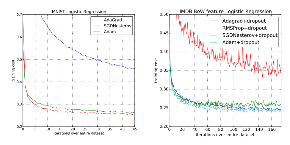
  • ADAM is much more robust to learning rate choices

  • ADAM is excellent when the gradient is sparse

  • ADAM is often the best in initial training stages

When is ADAM bad?

  • ADAM is perhaps the most widely used optimizer, the default for deep learning
  • However, it is not even guaranteed to converge on convex problems!
  • Can generalize worse (need more regularization)
  • Less memory efficient
  • It is very heuristic in nature, can be improved
  • You will explore benefits and drawbacks on your HW

Thanks!