DATA 609 Meetup 9: Convex Optimization Problems

George I. Hagstrom

Week Summary

  • Topic this week is convex optimization problems
  • Chapter 4.1, 4.2, 4.7 (we’ve sort of covered some of it)
  • Chapters 4.3-4.6 mostly useful for examples on first read (skim)
  • Read about solvers
  • Lab 5 available
  • Keep your eyes open for projects

Before we start, log-concave

  • Variety of generalizations of convexity
    • quasiconvex/quasiconcave
    • convexity w.r.t. a generalized inequality
  • For Stats and ML, log-concavity is very important
  • \(f(x)\) is log-concave if \(\log(f(x))\) is concave
    • Requires \(f(x) > 0\)
  • There is also log-convexity, but doesn’t arise

Stats Examples

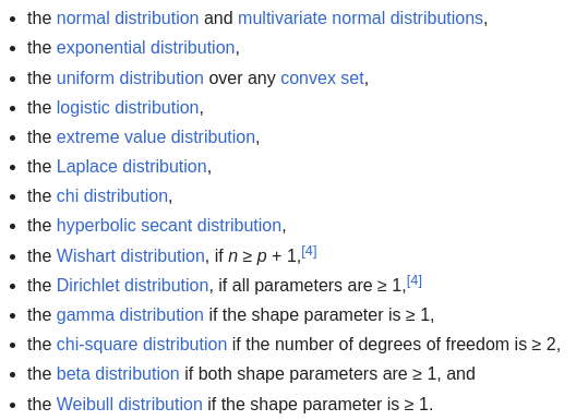
  • Many probability density functions are log-concave:
    • Normal distribution: \(\log(e^{-x^2}) = -x^2\)
    • Exponential distribution \(\log(e^{-\alpha x}) = -\alpha x\)
    • All from exponential family: \[ p(x|\theta) = \exp\left(\sum_{i=1}^s\nu_i(\theta)T_i(x) - A(\theta)\right)h(x) \]

Stats Examples

  • Incomplete list:

wikipedia

Marginalization/Partial Integration

  • If \(f(\mathbf{x},\mathbf{y})\) is log-concave, then so is: \[ g(\mathbf{x}) = \int \mathbf{dy} f(\mathbf{x},\mathbf{y}) \]
  • \(p(\mathbf{x},\mathbf{y})\) is log-concave then so is \(p(\mathbf{x}) = \int\mathbf{dy} p(\mathbf{x},\mathbf{y})\)

Convolution

  • Addition of two random variables is done by convolution:
  • \(z = x+y\) \[ p_{z}(z) = \int dx p_x(x)p_y(z-x) = p_x * p_y (z) \]
  • Convolution of two log-concave functions is log-concave

Cumulative Distribution Functions

  • CDF is probability random variable less than \(x\): \[ F(x) = \int_{-\infty}^x dx'p(x') \]
  • This is log-concave if \(p\) is log-concave
  • Also true for multidimensional CDF

Properties of log-concave

  • Products of log-concave are log-concave
    • \(f(\mathbf{x})g(\mathbf{x})\)
  • Sums are not (but are for log-convex)
  • Alternate definition: \(f(x)\) is log-convex if: \[ f(\theta x + (1-\theta)y) \geq f(x)^{\theta} f(y)^{1-\theta} \]
  • More technical: Moment and cumulant generating functions of log-concave density are log-concave

Example: Manufacturing Yield

  • You have a factory manufacturing some product
    • Bicycles, Wheels, Aluminum Rods, Magnets for MRI machines, etc
  • Each completed item is described by a set of parameters \(\theta\)
    • The roundness of the wheels
    • Thickness of bicycle tubes
    • Strength of rods/magnets
  • There is a set \(S\) which describes acceptable items, \(\theta\in S\) is item is well made

Manufacturing Yield

  • Suppose that your factory tries to build items with a target set of paramters \(x\)

  • Randomness/Imprecision causes manufactured items to deviate from target according to probability distribution: \[ p(\theta = x + w ) = p(w) \]

  • Then yield is defined as fraction of items within tolerances: \[ Y(x) = \int dw I(S,w+\theta) p(w) \]

Manufacturing Yield

  • Suppose you want to achieve a certain yield
  • If \(S\) is convex, and \(p\) log-concave, then consider: \[ C = \{x | Y(x) \geq \alpha \} = \{x | \log(Y(x)) \geq \log(\alpha) \} \]
  • C is a convex set (super-level set of a convex function)

Optimization Lingo

  • Covered some already
    • feasible points satisfy constraints
    • optimal value \(p^{\star}\) is tightest lower bound objective
    • optimal point is \(\mathbf{x}\) where \(f(\mathbf{x}) = p^{\star}\)
  • Some not:
    • infeasible: We say \(p^{\star}=\infty\) if we can’t find a single feasible point
    • unbounded below: We say \(p^{\star} = -\infty\) if objective doesn’t have lower bound

Implicit Constraints

  • Domain of objective \(f\) and constraint functions is included implicitly in constraints
  • i.e. \(\min_{x} f(x) = x\log(x)\) has implicit constraint \(x > 0\)
  • If no explicit constraints problem is called unconstrained

Slack or Active Inequality Constraints

  • Consider: \[ \min_{\mathbf{x}} f(\mathbf{x}) \\ g_i(\mathbf{x}) \leq 0 \]
  • Let \(x_{\mathrm{opt}}\) be optimal point
  • If \(g_i(x_{\mathrm{opt}}) < 0\) inequality \(i\) is slack
  • If \(g_i(x_{\mathrm{opt}}) = 0\) inequality \(i\) is active

Transforming Optimization Problems

  • We say that two (not necessarily convex) optimization problems are equivalent if we have a way to calculate the optimum of one problem from the solution of another problem

    • Monotone Transformation of Objective
    • Invertible Transformation of variables
    • Partial Minimization
    • Elimination of Equality Constraints
    • Introduction of Slack Variables

Transformation by monotone

  • Transformation by monotone increasing function \(h\) \[ \mathrm{argmin}_{x} h(f(x)) = \mathrm{argmin}_{x} f(x) \]
  • log is standard example
    • ML problems only convex once you take the log

Transform the variables

  • Suppose we have a one-to-one transformation \(x_i = \{\phi_i(\mathbf{z})\}\)
  • Then can substitute directly into objective and constraints: \[ \min_{\mathbf{z}} f(\phi(\mathbf{z})) \\ g_i(\phi(\mathbf{z})) \leq 0 \\ h_j(\phi(\mathbf{z})) = 0 \]

Transform the variables

  • Suppose you have a bilinear objective or constraint \[ xy \leq \alpha \]
  • Take log (monotone):
  • \(\log(x) + \log(y)\leq \log(\alpha)\)
  • \(z_1 = \log(x)\),\(z_2 = \log(y)\),
  • Leads to \(z_1+z_2\leq\log(\alpha)\)

Example: Geometric Programming

  • monomial: \(f(\mathbf{x}) = cx_1^{a_1}x_2^{a_2}\cdots x_n^{a_n}\)
  • posynomial: sum of monomials
  • Geometric Program: \[ \min_{\mathbf{x}} f_0(\mathbf{x}) \\ g_i(\mathbf{x}) \leq 1,\quad h_j(\mathbf{x}) = 1 \]
  • \(f\), \(g_i\) posynomials, \(h_j\) monomials

Geometric Programming

  • Can transform to convex problem by: \(y_i = \log(x_i)\), taking \(\log\) of objectives and constraints: \[ \min_{\mathbf{y}} \hat{f_0}(\mathbf{y}) = \log\left(\sum_k e^{\mathbf{a}_{0k}^T\mathbf{y}+b_{0k}} \right) \\ \hat{g_i}(\mathbf{y}) = \log\left(\sum_k e^{\mathbf{a}_{ik}^T\mathbf{y}+b_{ik}} \right) \\ \mathbf{h}_k^T\mathbf{y} + d_i = 0 \]

Partial Minimization

  • You can minimize with respect to some of the variables \[ \min_{x,y} f(x,y) = \min_x \hat{f}(x), \]
  • where \(\hat{f}(x) = \min_y f(x,y)\)
  • Constraints at each step depend on \(x\)
  • Can be life-saver, also preserves convexity

The other transformations

  • Mostly useful for making fast algorithms
  • Eliminating linear equality constraints by solving matrix equation
  • Eliminating linear inequalities with slack variables
  • Switching to epigraph form

Multicriterion Optimization

  • Often you need to balance multiple competing objectives:
    • For example, if you are building a car, you might care about minimizing the cost and maximizing the crash test rating or the reliability
    • If you are investing, you want to maximize the return, but minimize the chance of a catastrophic loss
    • If you are taking a political position, you want to appeal to the needs of different groups with distinct opinions

Multicriterion Optimization

\[ \min_{\mathbf{x}} \left(f_1(\mathbf{x}),f_2(\mathbf{x}),\cdots,f_n(\mathbf{x}\right)) \\ g_i(\mathbf{x}) \leq 0,\quad h_j(\mathbf{x}) = 0 \] - Feasible \(x\) that minimizes all objectives is an optimal point - Generally impossible - If possible objectives are called non-competing

Pareto Optimal

  • Consider a feasible point \(\mathbf{x}_1\)
  • \(\mathbf{x}_1\) dominates \(\mathbf{x}_2\) if at least matches \(\mathbf{x}_2\) on all objectives: \[ f_i(\mathbf{x}_1)\leq f_i(\mathbf{x}_2) \]
  • and beats it on one \(f_j(\mathbf{x}_1) < f_j(\mathbf{x}_2)\)
  • Two cars that are identical except one is cheaper
  • A point \(\mathbf{x}\) is Pareto optimal if it is dominated by no other points
  • You can make a case for a Pareto optimal points

Pareto Front

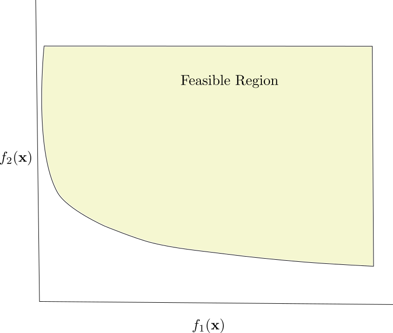
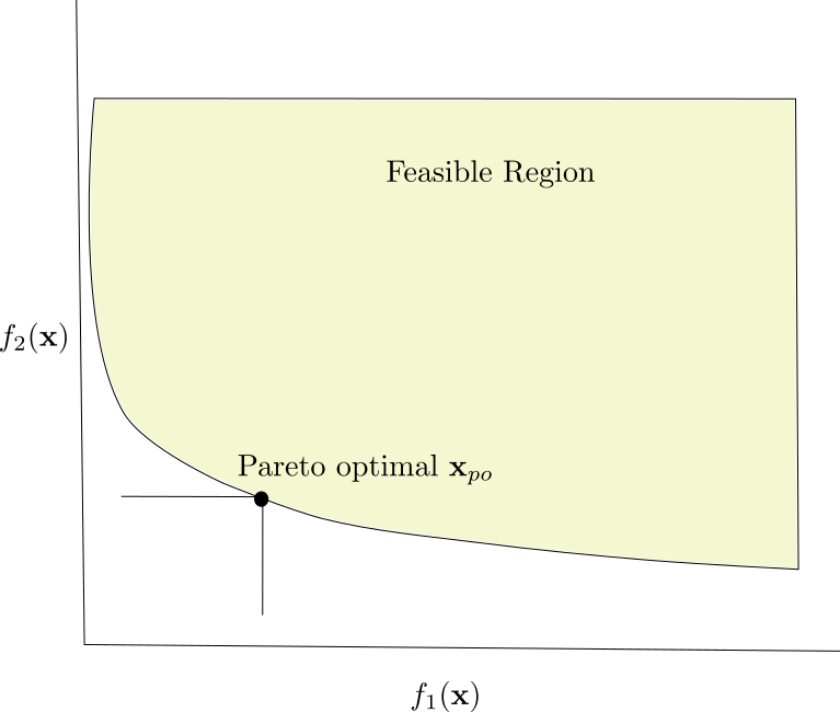
  • Graph the competing objective functions

Pareto Front

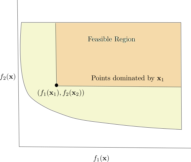
  • Dominated points are above and to right of focal point

Pareto Front

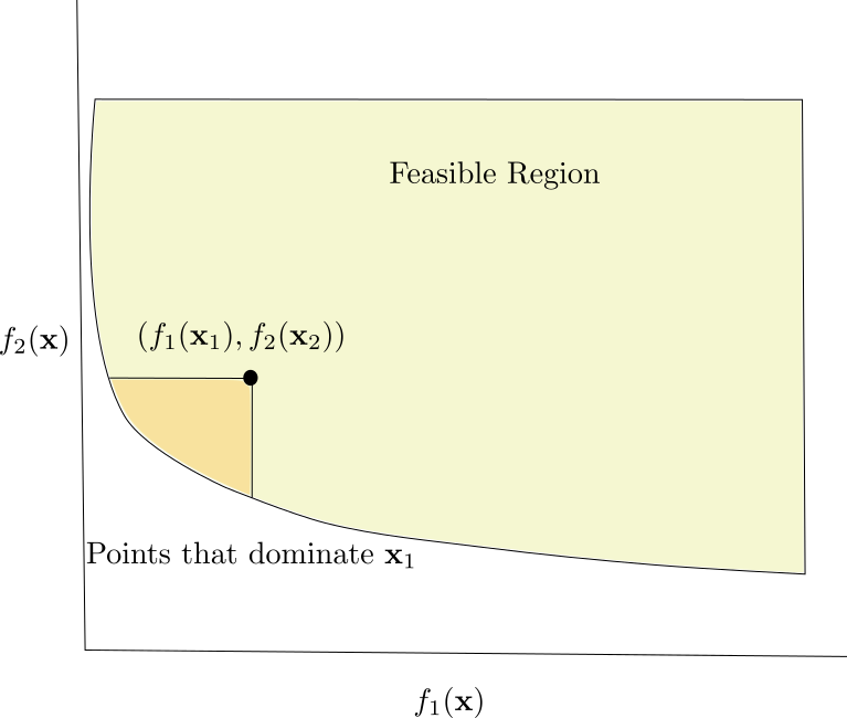
  • Focal point dominated by points down and left

Pareto Front

  • Pareto Front is Pareto Optimal points

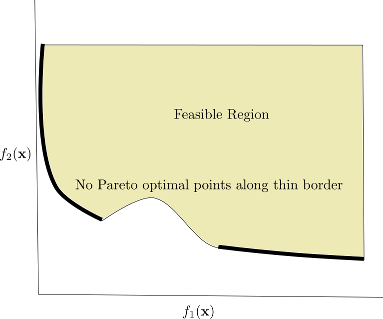
Pareto Front

  • Boundary not necessarily a Pareto front

Scalarization

  • Can add multiple objectives up to create a standard optimization problem \[ \min_{\mathbf{x}} \sum_k \lambda_k f_k(\mathbf{x}) \]
  • \(\lambda_k\) convert between each objective function to the same units and define trade-offs
  • Always finds a Pareto Optimal point

Ridge Regression Trade Off

Text(0, 0.5, 'Mean Square Error')
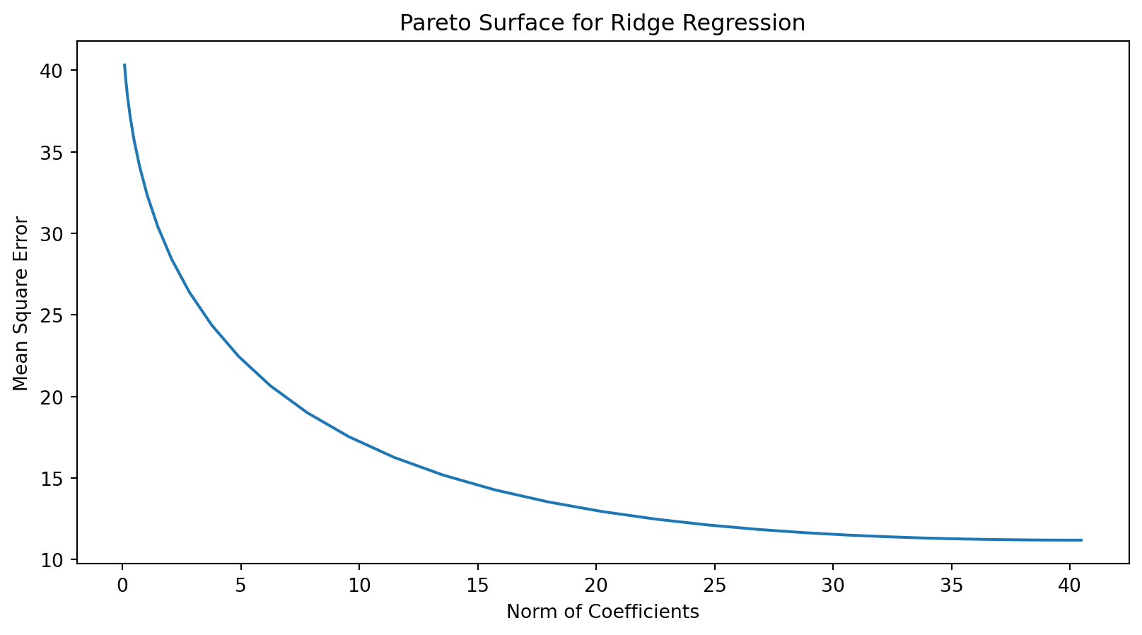
Ridge Regression Trade Off

for v in lambd_values:
    lambd.value = v
    problem.solve()
    train_errors.append(mse(X_train, Y_train, beta))
    test_errors.append(mse(X_test, Y_test, beta))
    beta_values.append(beta.value)
    
norm_beta_vec = np.array([np.linalg.norm(vec)**2 for vec in beta_values])  
plt.plot(norm_beta_vec,train_errors)
plt.title("Pareto Surface for Ridge Regression")
plt.xlabel("Norm of Coefficients")
plt.ylabel("Mean Square Error")

CVX Solvers

  • Just like other software packages, CVX has a number of different solvers
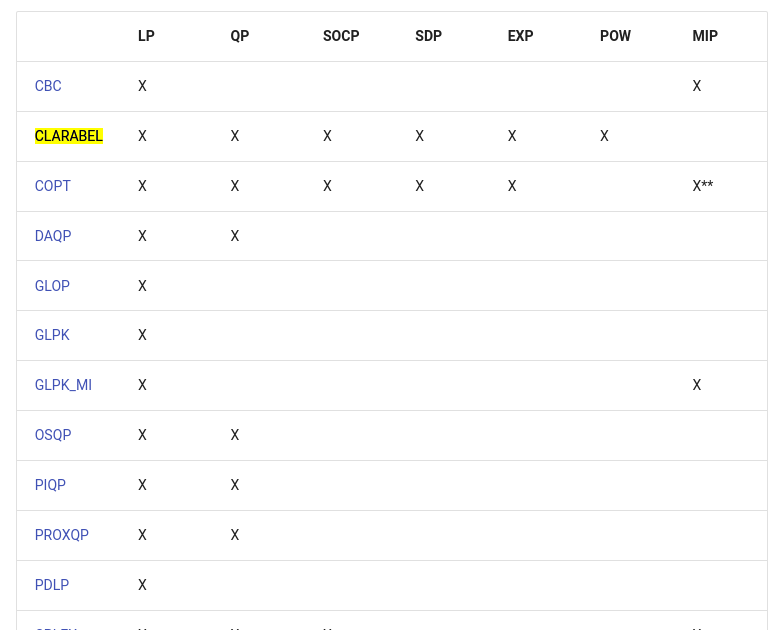
  • Three free solvers: SCS, CLARABEL, OSQP
  • SCS is the in-house solver (Splitting Conic Solver)
  • OSQP from Oxford, does LP and QP
  • CLARABEL from Oxford specializes in Second Order Cone Programs

Choosing a Solver

  • CVX can pick by default
  • Or you can specify
import CVYPY as cvx
cvx.solve(solver="CLARABEL", 
verbose=False, 
gp=False, qcp=False,
requires_grad=False, 
enforce_dpp=False, 
ignore_dpp=False, **kwargs)

Not all Solvers can Solve all Problems

Warm Start

  • If you are solving many versions of the same problem, CVX by default caches results of computation and uses them as starting point
  • Leads to a big speed up

Other Solvers I’ve Used

  • MOSEK commercial nonlinear solver, some universities have a license/possible to get academic license
  • GUROBI fastest for linear programming
  • GLPK solver of last resort in some python packages when your MOSEK license isn’t working
Thanks!