DATA 622 Meetup 11: Interpretable ML
2026-04-13
Data Science Seminar Tomorrow!!!
HW 4 Comments
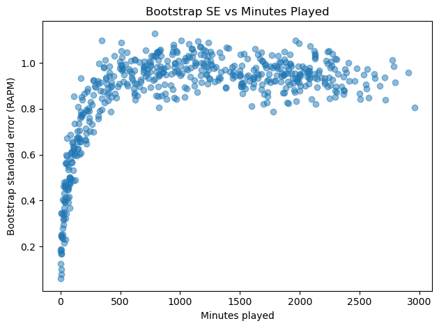
- Interpreting Graphs
- Bootstrap Uncertainty vs Minutes Played
HW 4
- Interpreting Graphs
- Bootstrap Uncertainty vs Minutes Played
Is uncertainty is highest for low minute players?
Black Boxes Gone Wrong
- Clever Hans: Horse that could add
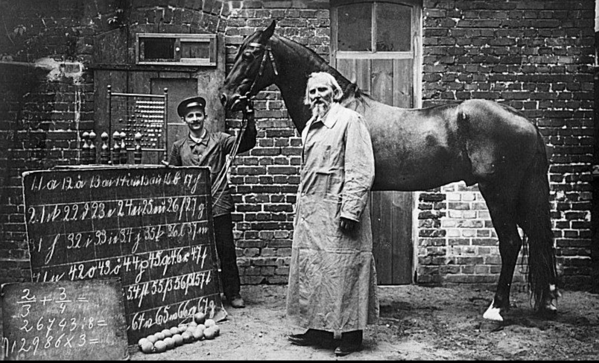
wikipedia
Black Boxes Gone Wrong
- Dog vs. Wolf


- Image classifier trained on images of dogs and wolves used the presence of snow as primary means of determining class
Black Boxes Gone Wrong
- Identifying Whales in Hydrophone Recordings
- Cornell University held a contest to identify Right Whales
![]()

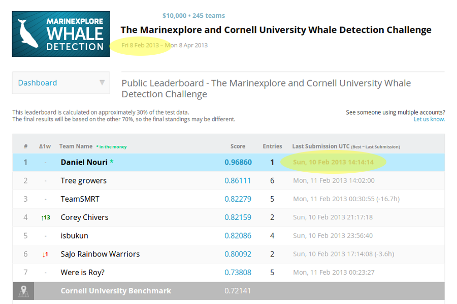
Black Boxes Gone Wrong
- Identifying Whales in Hydrophone Recordings
- Cornell University held a contest to identify Right Whales
- Winner had astonishingly high accuracy
When Interpretability?
- Sometimes the reasons are critical
- Detecting pedestrians or cyclists in self-driving cars


Interpretability Methods
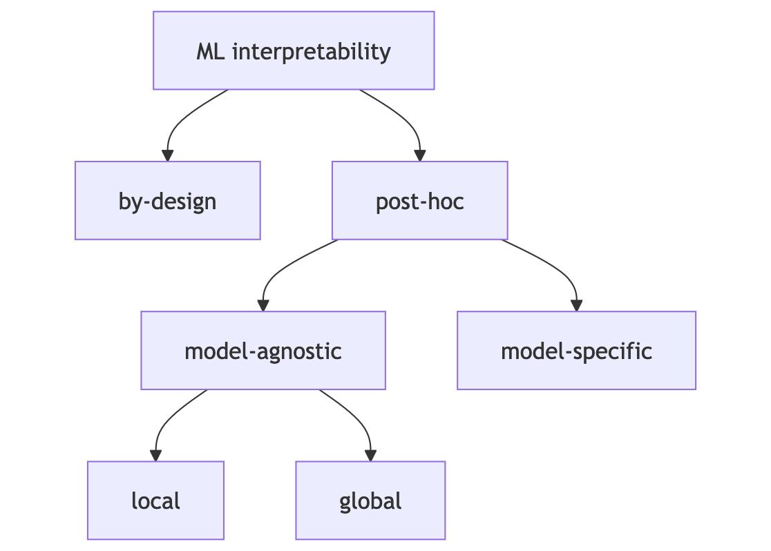
ML Interpretability
Interpretability Methods
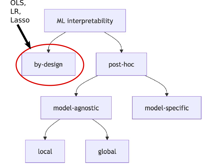
ML Interpretability
Interpretability Methods
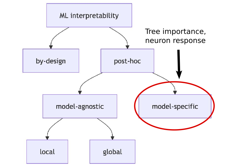
ML Interpretability
Interpretability Methods
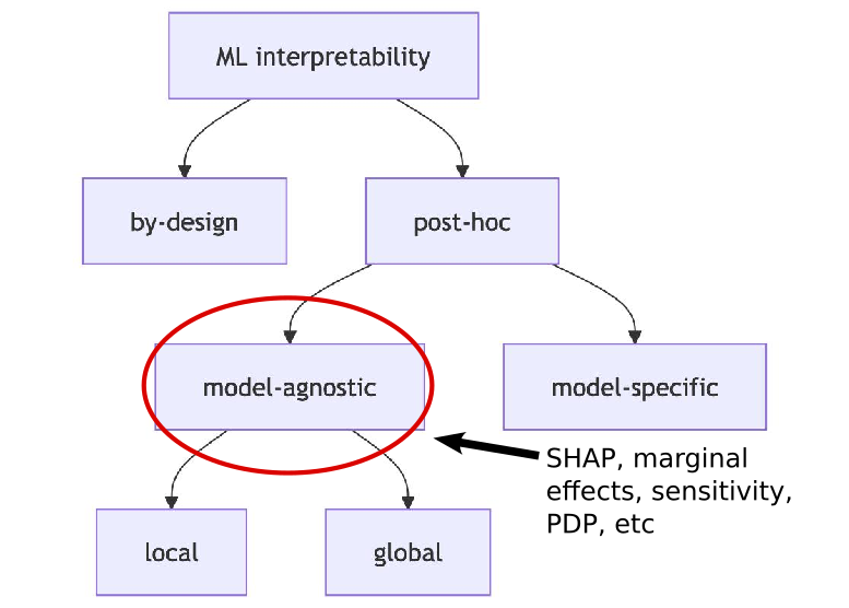
ML Interpretability
Bikeshare Model by Hour
- Let’s look at the predictive accuracy by hour
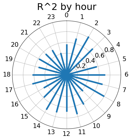
Bikeshare Model by Hour
- Let’s look at the predictive accuracy by hour

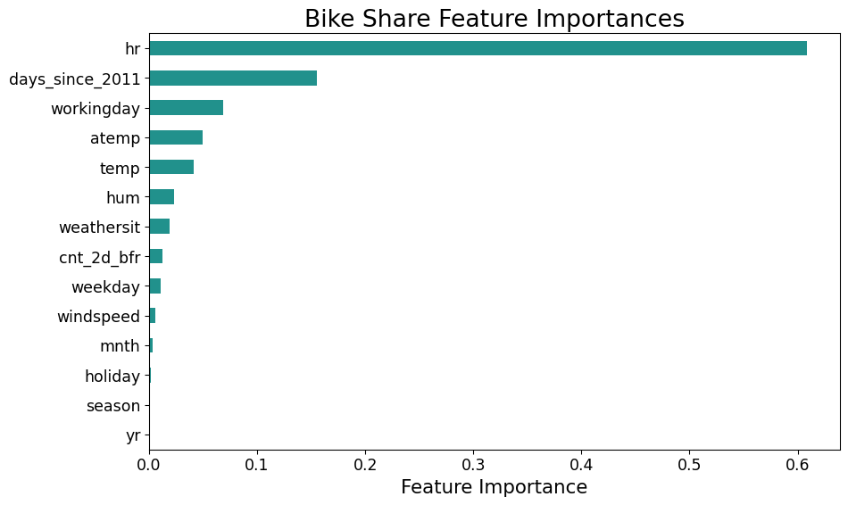
Tree Importance
Local Versus Global
- Local looks at the impact of features at a specific data point.
- Ceteris Parabis plots (or “Slope” or “Marginal Effect”):
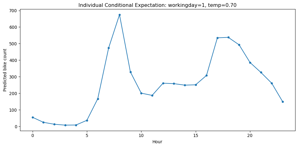
Local Versus Global
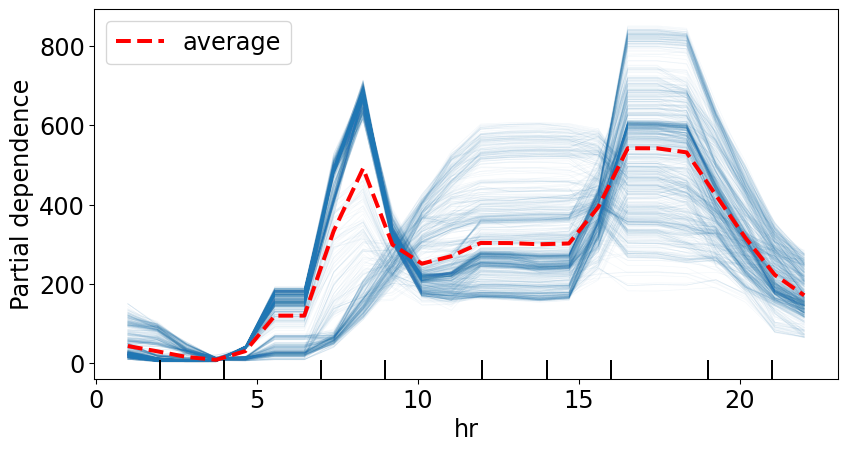
- Global looks at the impact of the feature averaged over many instances
- Partial Dependence Plot averages all of the Conditional Expectation Curves
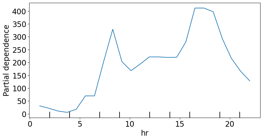
Local Versus Global
- Global looks at the impact of the feature averaged over many instances
- Partial Dependence Plot averages all of the Conditional Expectation Curves
Shapley Example
- Our data point is 50\(m^2\), 1st floor, bans cats, near parks
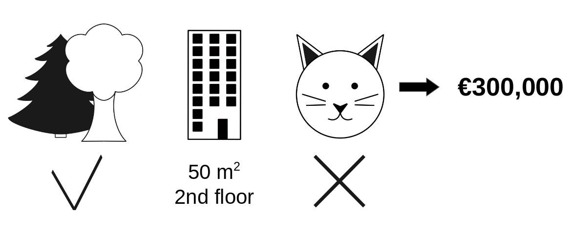
molnar 17
Shapley Example
- Consider full coalition
- Just look at difference between ban cats and not
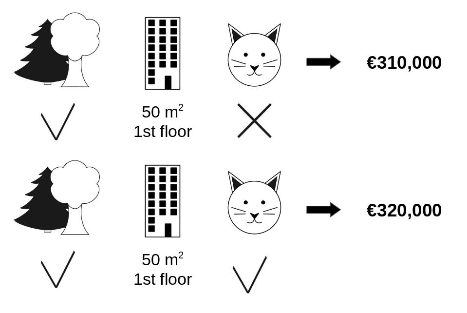
molnar 17
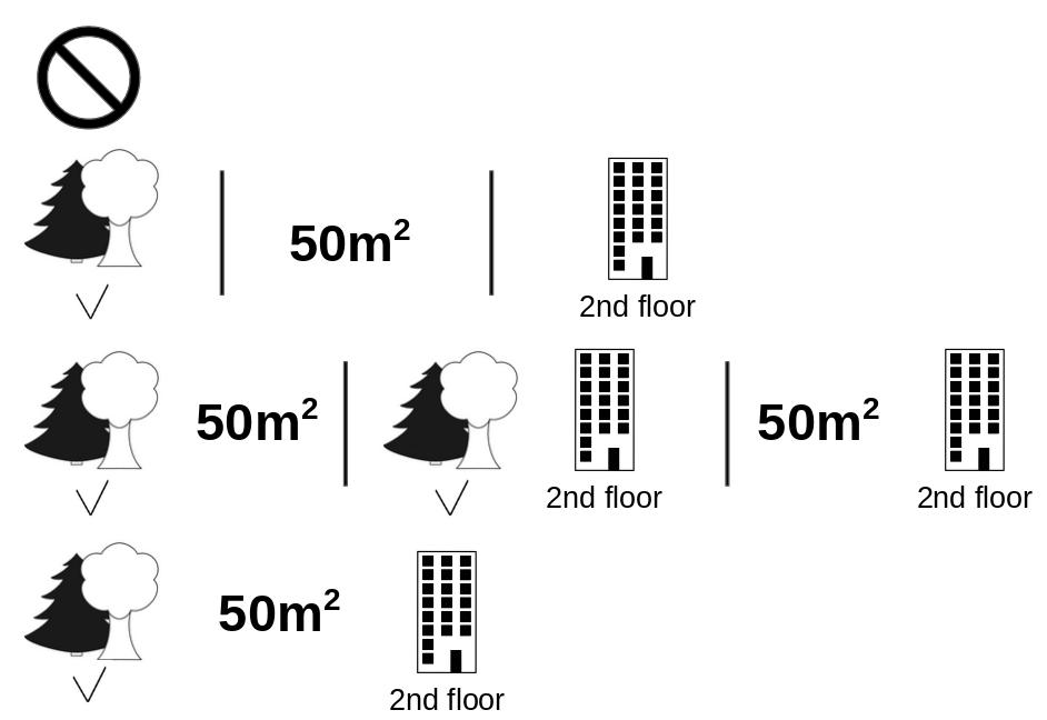
Shapley Coalitions
- Here are all the coalitions behind a single shapley value
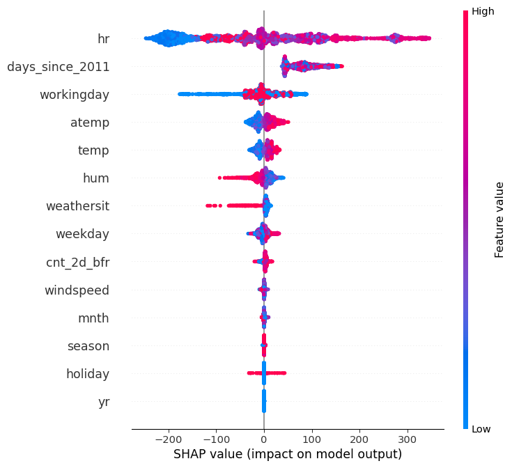
SHAP Importance
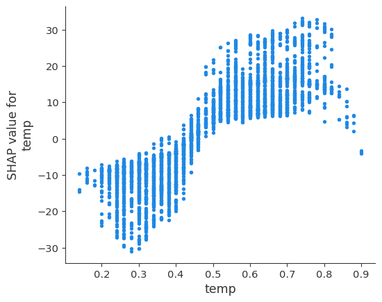
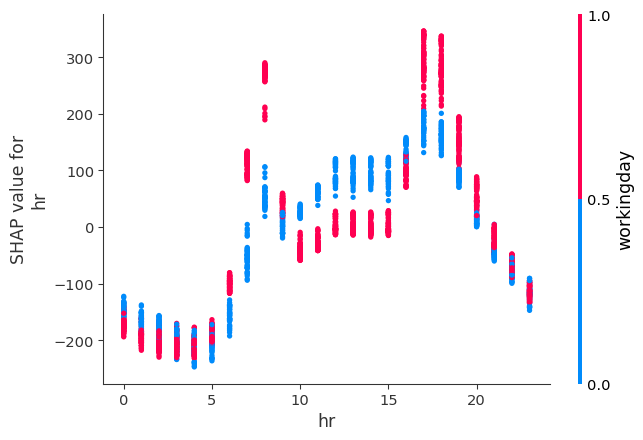
SHAP Dependence Plot
Interactions by default
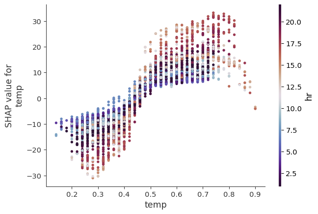
SHAP Interactions Plot
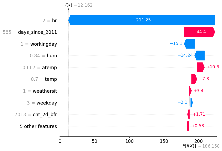
Shap Waterfall Plot
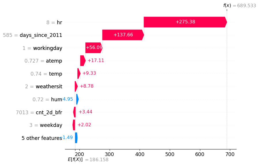
Shap Waterfall Plot v2
Shap Plot for the worst prediction
2012-12-27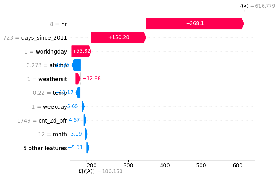
Thanks!
![]()