DATA 622 Meetup 12: Neural Networks

George I. Hagstrom

2026-04-20

Week Summary

• Contact me ASAP if you haven’t scheduled MVP demo
• Lab 7 due Sunday May 3rd
• You will want a Google Colab Pro student account!!!
• Vignette on neural networks in Colab

Neural Network Gameplan

• Week 12: Basics, pytorch, activation functions, optimization algos
• Week 13: CNNs, RNNs, Deep Learning Considerations, vision applications
• Week 14: Pretrained Networks, Transfer Learning, text applications

Introduction to Neural Networks

• Invented originally to understand how the brain works

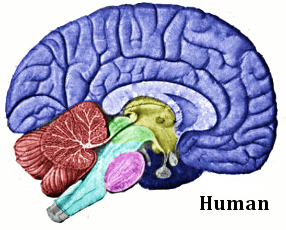
Source: wikipedia

Introduction to Neural Networks

• Was found to have an enormous number of applications
  • Classification
  • Pattern Recognition
  • Generative Models

Introduction to Neural Networks

• Interesting objects in their own right
  • People study them as they would any other complex systems

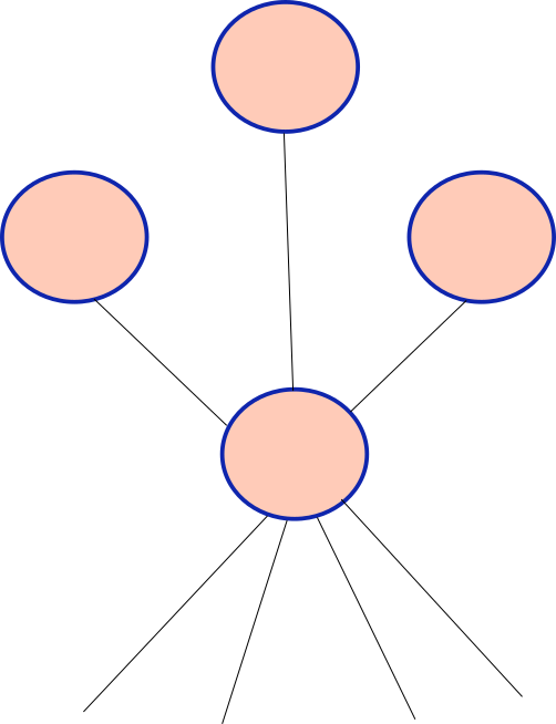
What is a Neuron?

• Neurons send and receive electrical signals

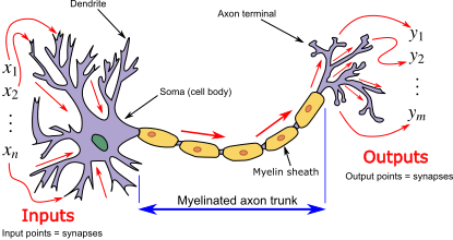
wikipedia

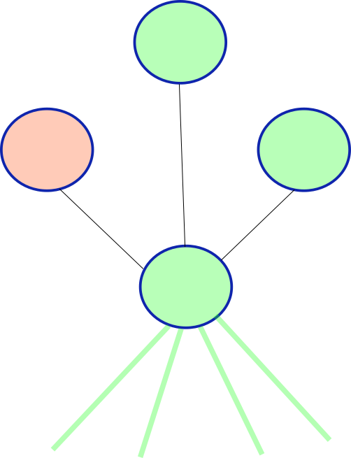
Connected Neurons

• They are connected to other neurons

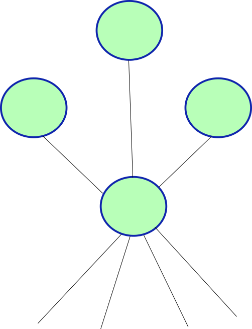
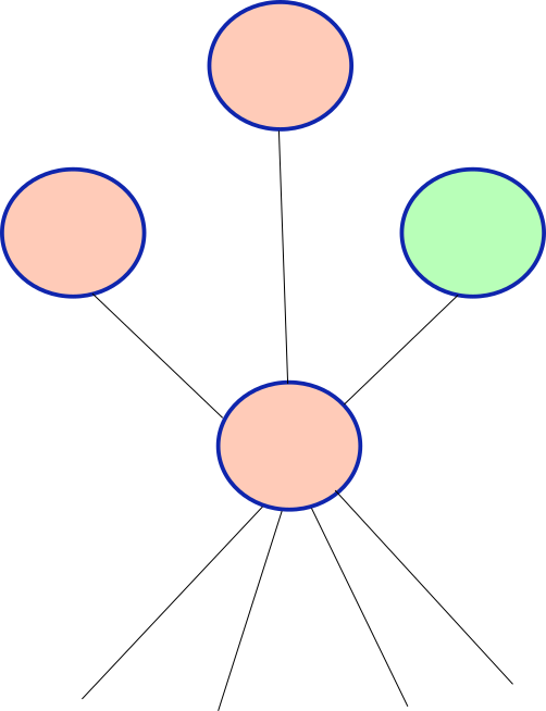
Connected Neurons

• They are connected to other neurons
• They respond to stimulus from senses and other neurons

Connected Neurons

• They are connected to other neurons
• They respond to stimulus from senses and other neurons

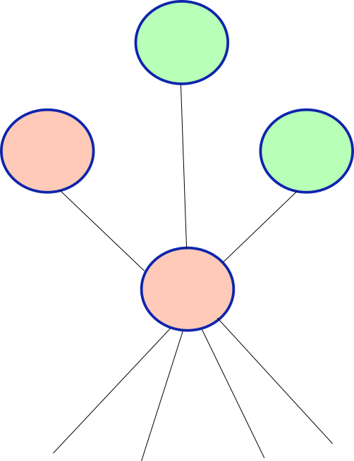
Connected Neurons

• They are connected to other neurons
• They respond to stimulus from senses and other neurons
• Cross a threshold before firing

Connected Neurons

• They are connected to other neurons
• They respond to stimulus from senses and other neurons
• Cross a threshold before firing

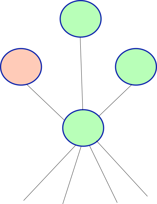
Connected Neurons

• They are connected to other neurons
• They respond to stimulus from senses and other neurons
• Cross a threshold before firing
• Neuronal Cascade is part of cognition

Single Neuron

• Single Neuron converts several inputs into an output:

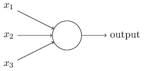
Nielson

Single Neuron

• Integrates over the input signals using weights: \[ x_{\mathrm{out}} = \phi\left(\sum_{i=1}^n w_ix_i + c\right) \]

Single Neuron

• Integrates over the input signals using weights: \[ x_{\mathrm{out}} = \phi\left(\sum_{i=1}^n w_ix_i + c\right) \]

• \(\phi\) is called the activation function

• \(w_i\) are the weights

• \(c\) is the bias

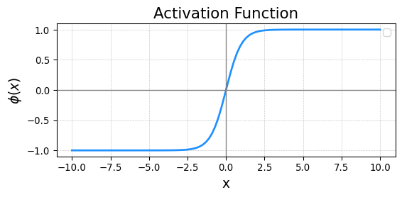
Activation Functions

• Biology intuition:
  • \(\phi=1\) when integrated inputs positive
  • \(\phi=0\) or \(\phi=-1\) (doesn’t matter) when integrated input negative
• Leads to step/sigmoid functions:

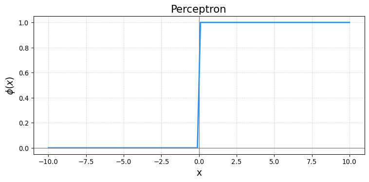
Activation Functions to Know

• Perceptron \[ \phi(x) = \cases{1& \text{if} \quad x\geq 0 \\ 0& \text{if} \quad x<0} \]

Activation Functions to Know

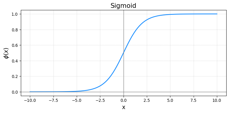
• Sigmoid Function

\[ \phi(x) = \frac{1}{1+e^{-x}} \]

Activation Functions to Know

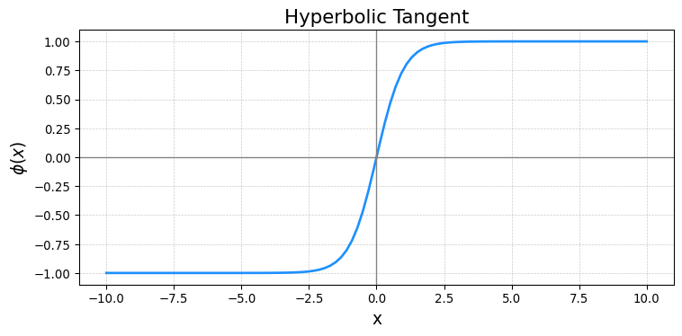
• Hyperbolic Tangent

\[ \phi(x) = \frac{e^x - e^{-x}}{e^x +e^{-x}} \]

Activation Functions to Know

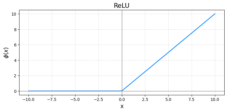
• Rectified Linear Unit (ReLU)

\[ \phi(x) = \cases{0& \text{if} \quad x\geq 0 \\ x& \text{if} \quad x<0} \]

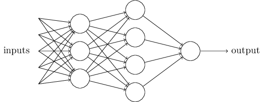
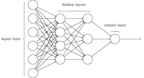
Feedforward Neural Networks

• Input layer, one neuron per input variable
• One neuron per target function
• Neurons organized in layers

Feedforward Examples

• Image Recognition
  • Input Neurons are pixels
  • Output neurons correspond to each category
  • Inner Layers Represent Features
  • Can use a softmax layer at the end to determine category

Neural Network Considerations

• Even a small NN can be huge:

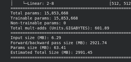
• Need lots of data
• Lots of different regularization

What are NNs used for?

• Anything where the features are abstract
  • Images
  • Audio
  • Text
• Large amounts of data
• Tabular data problems decision trees often just as good but with less trouble

How would you train one?

• Have set of training data \(\mathbf{x}_i\) and target \(y_i\)
• Have settled on an architecture:
  • \(n_i\) neurons in layer \(i\)
  • \(m\) total layers
  • \(w_{jk,i}\) is weight of neuron \(j\) in layer \(i-1\) on neuron \(k\) in layer \(i\)
  • \(b_{ki}\) is bias of neuron \(k\) in layer \(i\)

How would you train one?

• Overall neural network generates a function: \[ y_{\mathrm{pred}} = F(\mathbf{x}) \]
• Evaluate function by stepping through the layers in order
• Can define a loss minimization problem: \[ \min_{\mathbf{w},\mathbf{b}} \sum_{l=1}^N \Phi(y_l,F(\mathbf{x},\mathbf{w},\mathbf{b})) \]

Backpropagation

• In order to optimize, compute the gradient
• Repeated application of the chain rule
• NN packages use the network structure to efficiently compute the gradients
• Referred to as backpropagation
• Related technique of automatic differentiation

pytorch

• Open Source Machine Learning Library from Meta/FB
• PyTorch optimizes usability while maintaining good performance
  • No small task when dealing with GPUs
• PyTorch favors simple over easy
  • A little bit harder at first when working with GPUs
  • But easier to debug when you build complex models
• Python First

tensors

• Primary data object in pytorch is called a tensor

import torch
import numpy as np

data = [[1, 2],[3, 4]]
x_data = torch.tensor(data)
x_data

tensor([[1, 2],
        [3, 4]])

tensors

• Tensors are like magic numpy arrays
  • They live on a particular device:

print(f"Device tensor is stored on: {x_data.device}")

Device tensor is stored on: cpu

• When programming with GPUs, you must manually control the movement of tensor data across the cluster

What is a GPU

• Normal computers have several (~20) very powerful cores
  • Each core can do complex operations sequentially
• GPU has huge number (~10,000) of very basic cores
  • Cores can just multiply and add
  • Cores work in parallel
  • Perfect for Neural Networks

tensors

• Tensors are like magic numpy arrays
  • They come with automatic gradient tracking
  • When you perform a computation with a tensor, pytorch stores the computational graph
  • *.backward() computes gradient

x = torch.ones(5)  # input tensor
y = torch.zeros(3)  # expected output
w = torch.randn(5, 3, requires_grad=True)
b = torch.randn(3, requires_grad=True)
z = torch.matmul(x, w)+b
loss = torch.nn.functional.binary_cross_entropy_with_logits(z, y)

loss.backward()

tensors

• loss.backward() updated the tensors w and b to include the gradient with respect to loss \[ \frac{\partial \mathrm{loss}}{\partial \mathbf{w}},\quad \frac{\partial \mathrm{loss}}{\partial \mathbf{b}}, \]

print(w.grad)
print(b.grad)

tensor([[0.0065, 0.3193, 0.2655],
        [0.0065, 0.3193, 0.2655],
        [0.0065, 0.3193, 0.2655],
        [0.0065, 0.3193, 0.2655],
        [0.0065, 0.3193, 0.2655]])
tensor([0.0065, 0.3193, 0.2655])

Dataloaders

• pytorch is written to separate model building/training and dataset management
• torch.utils.data.Dataset enables built in datasets
• torch.utils.data.DataLoader is for managing and iterating over datasets

DataLoaders

• This code will download the fashion-mnist dataset and prep it for use:

import torch
from torch.utils.data import Dataset
from torchvision import datasets
from torchvision.transforms import ToTensor
import matplotlib.pyplot as plt


training_data = datasets.FashionMNIST(
    root="data",
    train=True,
    download=True,
    transform=ToTensor()
)

test_data = datasets.FashionMNIST(
    root="data",
    train=False,
    download=True,
    transform=ToTensor()
)

Constructing a Neural Network

• Neural Network architectures are constructed using the nn.Module class

import torch.nn as nn
import torch.nn.functional as F
import torch.optim as optim


# The network class contains the intializer and some methods for our neural network
# You create a network by calling Network([Nodes_Input,Nodes_2,Nodes_3,...,Nodes_Output]) 

class Network(nn.Module):
    def __init__(self, sizes):
        super(Network, self).__init__()
        self.sizes = sizes
        self.num_layers = len(sizes)
        
        self.layers = nn.ModuleList()
        for i in range(self.num_layers - 1):
            layer = nn.Linear(sizes[i], sizes[i+1])
            nn.init.xavier_normal_(layer.weight)   # Good initialization for shallow/sigmoid nets
            #nn.init.kaiming_normal_(layer.weight, mode='fan_out', nonlinearity='relu') initialization for relus
            #nn.init.kaiming_uniform_(layer.weight, mode='fan_out', nonlinearity='relu') initialization for relus and deep nets

            nn.init.zeros_(layer.bias)               # initialize the bias to 0
            self.layers.append(layer)
    
    # Forward is the method that calculates the value of the neural network. Basically we recursively apply the activations in each
    # layer
    
    def forward(self, x):
        for layer in self.layers[:-1]:
            x = nn.sigmoid(layer(x))   # sigmoid layers
            #x = F.relu(layer(x)) # You will try the relu layer in the last problem
        x = self.layers[-1](x) 
        return x

Initializing a Network

• Can call the constructor to make your network:

Network([784,100,10])

Network(
  (layers): ModuleList(
    (0): Linear(in_features=784, out_features=100, bias=True)
    (1): Linear(in_features=100, out_features=10, bias=True)
  )
)

Training a network

• Define Training Function

def train(network, train_data, epochs, eta, test_data=None):
 
    optimizer = optim.SGD(network.parameters(),momentum=0.8,nesterov=True, lr=eta,weight_decay=1e-5)
    loss_fn = nn.CrossEntropyLoss()
    
    loss_history = []      
    accuracy_history = []  
    train_accuracy_history = []

    # We are going to loop over the epochs
    for epoch in range(epochs):
        # This puts the network into training mode
        network.train()
        running_loss = 0.0
        batch_count = 0

Training a Network

• Loop over batches of training examples

        # Now we loop through the batches to train
        for data, target in train_data:
            optimizer.zero_grad() # This clears the internally stored gradients
            output = network(data) # evaluate the neural network on the minibatch, we will compare this to the target
            # Here we calculate the loss function and then use backpropagation
            # to calculate the gradient
            loss = loss_fn(output, target) 
            loss.backward()
        
            # Update the weights
            optimizer.step()
            
            running_loss += loss.item()
            batch_count += 1

Loading Data

from torchvision import datasets, transforms
from torch.utils.data import DataLoader

transform = transforms.Compose([transforms.ToTensor(), transforms.Lambda(lambda x: x.view(-1))])


train_dataset = datasets.FashionMNIST('data/', train=True, download=True, transform=transform)
test_dataset = datasets.FashionMNIST('data/', train=False, transform=transform)

img, label = training_data[100]

plt.imshow(img.squeeze(),cmap="gray")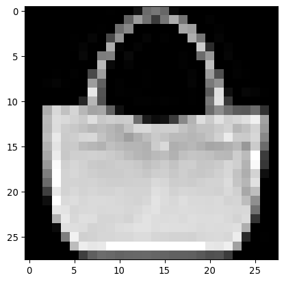

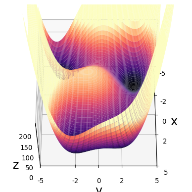
Train

train_loader = DataLoader(train_dataset, batch_size=10, shuffle=True)
test_loader = DataLoader(test_dataset, batch_size=10, shuffle=False)

# Initialize network
net = Network([784, 30, 10])

# Train
train(net, train_loader, epochs=1, eta=0.01, test_data=test_loader)

Optimization Basics

• Simplified loss landscape:
• Imagine more dimensions

Gradient Descent

• Start at \(\mathbf{x}_0\)
• Find gradient \(\nabla \mathrm{loss}(\mathbf{x})\)
• \(\mathbf{x}_n = \mathbf{x}_{n-1} - \kappa \nabla\mathrm{loss}(\mathbf{x}_{n-1})\)
• \(\kappa\) is learning rate

What Learning Rate to Pick?

• High learning rate trains faster
• Too high and don’t converge at all
• Limit is set by algorithm and ellipticity of well

What Learning Rate to Pick?

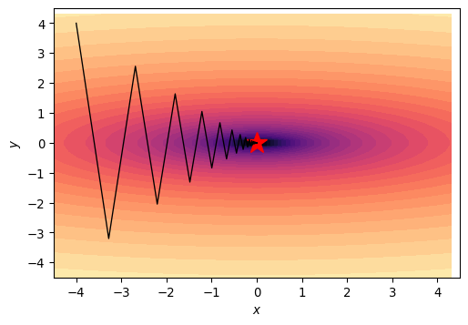
• Steepness discrepancy limits learning rate
• Most of the step is in wrong direction

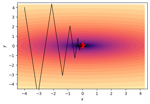
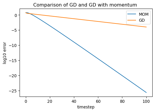
Momentum

• Advanced algos use momentum, gives “memory” of past gradient
• Reduces effect of valley oscillation

Hyperparameter Problems

• We don’t know the shape of the loss landscape to pick \(\kappa\)
• We handle this several ways:
  • Experimentation
  • Heuristics
  • Adaptive Methods

Stochastic Gradient Descent

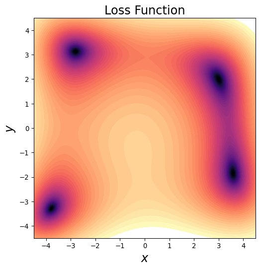
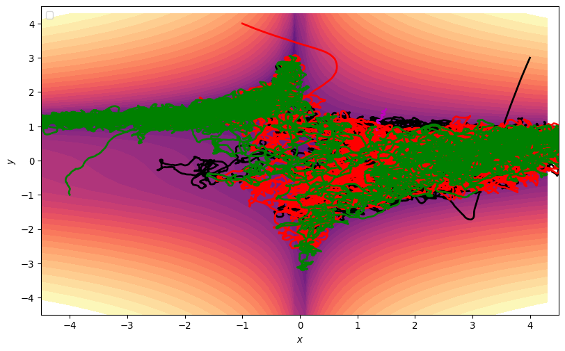
• Common for optimization algorithms to “get stuck”

Stochastic Gradient Descent

• In low-D local minima are problematic

Stochastic Gradient Descent

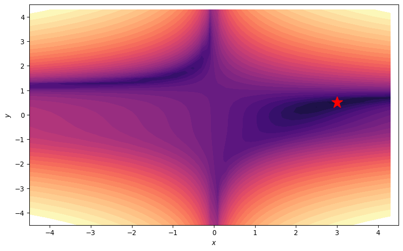
• Trajectories get Stuck

Stochastic Gradient Descent

• The barriers in high dimensions likely more complex
• Stochastic Gradient Descent modifies gradient descent style methods
  • Compute the gradient of loss using only part of the data
  • Called a “mini-batch”
  • Smaller the mini-batch, the more the noise

Stochastic Gradient Descent

Stochastic Gradient Descent

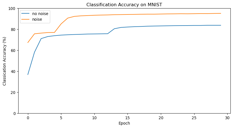
• In 2D, can just add noise

Annealing

• Noise can deflect you from the minimum when you are close
• Common practice is to start with noise high, reduce it later
  • Simulated annealing (from metallurgy)
• Even more common to start with high learning rate and gradually decrease it
  • Whereas in some ML applications increasing batch-size could cause overfitting

Adaptive Methods

• We saw that hyper-parameters are hard to pick at outset
• Ideal learning rate depends on condition number and also magnitude of gradients
• Concept: Change Learning Rate as we go
  • Keep memory of gradient in each variable
  • Step in the direction of the average gradient
  • Decrease learning rate if variance is high
  • Increase learning rate if variance is low

ADAM

• Adaptive Moment Estimation
• Have a local estimate of average gradient \(\hat{\mathbf{v}}_i\)
• Have a local estimate of squared gradient \(\hat{G}_{s,i}\)
• Adjusted learning rate based on both: \[ \mathbf{x}_{i+1} = \mathbf{x}_i -\kappa \frac{\hat{\mathbf{v}}_i}{\sqrt{\hat{G}_{s,i}+\epsilon}} \]

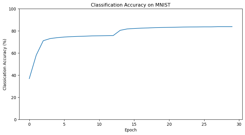
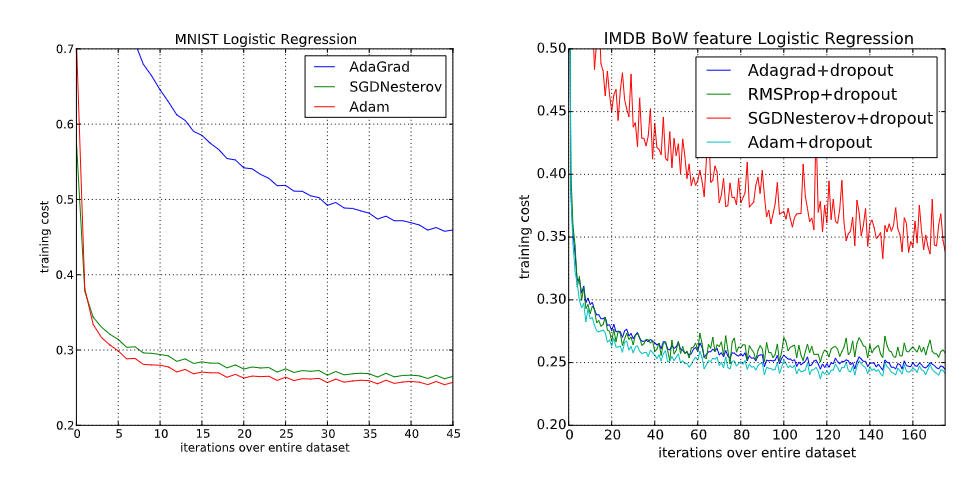
When and Why is ADAM good?

• ADAM is much more robust to learning rate choices

• ADAM is excellent when the gradient is sparse

• ADAM is often the best in initial training stages

When is ADAM bad?

• ADAM is perhaps the most widely used optimizer, the default for deep learning
• However, it is not even guaranteed to converge on easy problems
• Can generalize worse (need more regularization)
• Less memory efficient
• It is very heuristic in nature, can be improved

Thanks