DATA 622 Meetup 13: Neural Networks

George I. Hagstrom

2026-04-27

Week Summary

• Focus this week is convolutionary neural networks (CNNs)
• Secondary focus:
  • Heuristics for training Neural Networks
  • Deep Neural Network Issues
• Lab 7 Due this week

Optimization Basics

• Simplified loss landscape:
• Imagine more dimensions

Gradient Descent

• Start at \(\mathbf{x}_0\)
• Find gradient \(\nabla \mathrm{loss}(\mathbf{x})\)
• \(\mathbf{x}_n = \mathbf{x}_{n-1} - \kappa \nabla\mathrm{loss}(\mathbf{x}_{n-1})\)
• \(\kappa\) is learning rate

What Learning Rate to Pick?

• High learning rate trains faster
• Too high and don’t converge at all
• Limit is set by algorithm and ellipticity of well

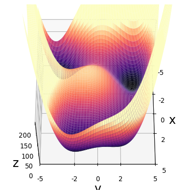
What Learning Rate to Pick?

• Steepness discrepancy limits learning rate
• Most of the step is in wrong direction

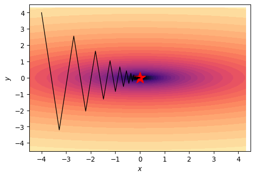
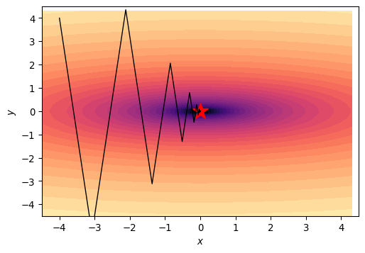
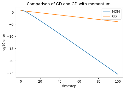
Momentum

• Advanced algos use momentum, gives “memory” of past gradient
• Reduces effect of valley oscillation

Hyperparameter Problems

• We don’t know the shape of the loss landscape to pick \(\kappa\)
• We handle this several ways:
  • Experimentation
  • Heuristics
  • Adaptive Methods

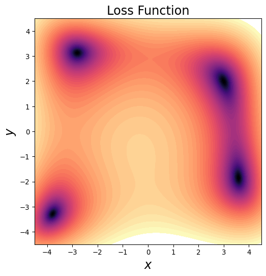
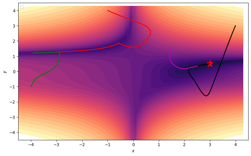
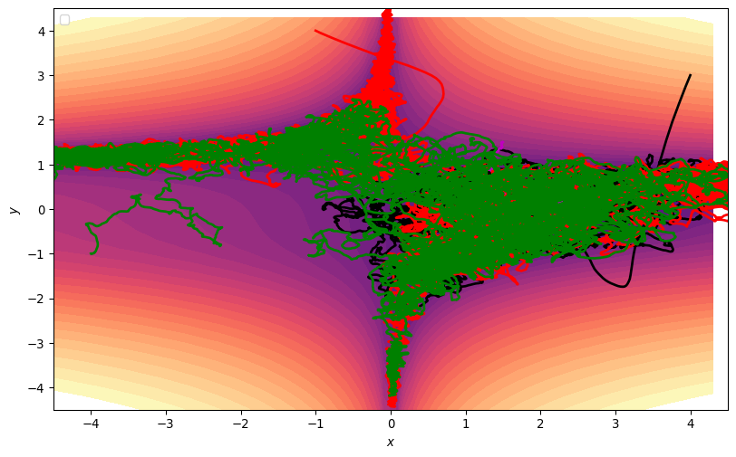
Stochastic Gradient Descent

• Common for optimization algorithms to “get stuck”

Stochastic Gradient Descent

• In low-D local minima are problematic

Stochastic Gradient Descent

• Trajectories get Stuck

Stochastic Gradient Descent

• The barriers in high dimensions likely more complex
• Stochastic Gradient Descent modifies gradient descent style methods
  • Compute the gradient of loss using only part of the data
  • Called a “mini-batch”
  • Smaller the mini-batch, the more the noise

Stochastic Gradient Descent

Stochastic Gradient Descent

• In 2D, can just add noise

Annealing

• Noise can deflect you from the minimum when you are close
• Common practice is to start with noise high, reduce it later
  • Simulated annealing (from metallurgy)
• Even more common to start with high learning rate and gradually decrease it
  • Whereas in some ML applications increasing batch-size could cause overfitting

Adaptive Methods

• We saw that hyper-parameters are hard to pick at outset
• Ideal learning rate depends on condition number and also magnitude of gradients
• Concept: Change Learning Rate as we go
  • Keep memory of gradient in each variable
  • Step in the direction of the average gradient
  • Decrease learning rate if variance is high
  • Increase learning rate if variance is low

ADAM

• Adaptive Moment Estimation
• Have a local estimate of average gradient \(\hat{\mathbf{v}}_i\)
• Have a local estimate of squared gradient \(\hat{G}_{s,i}\)
• Adjusted learning rate based on both: \[ \mathbf{x}_{i+1} = \mathbf{x}_i -\kappa \frac{\hat{\mathbf{v}}_i}{\sqrt{\hat{G}_{s,i}+\epsilon}} \]

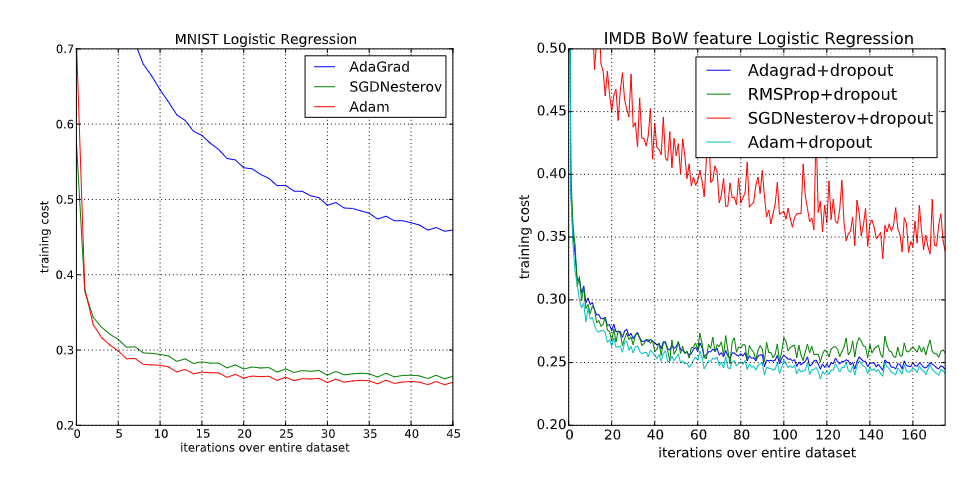
When and Why is ADAM good?

• ADAM is much more robust to learning rate choices

• ADAM is excellent when the gradient is sparse

• ADAM is often the best in initial training stages

When is ADAM bad?

• ADAM is perhaps the most widely used optimizer, the default for deep learning
• However, it is not even guaranteed to converge on easy problems
• Can generalize worse (need more regularization)
• Less memory efficient
• It is very heuristic in nature, can be improved

Inductive Bias

• Machine Learning works best when structure of hypothesis set matches structure of target function:
  • Linear regression and linear relationships
  • Naive Bayes and feature independence
  • Decisions Trees bias towards specific features
  • Nearest Neighbors: Features contribute equally

Network Architecture and Inductive Bias

• Fully Connected Networks don’t have much inductive bias

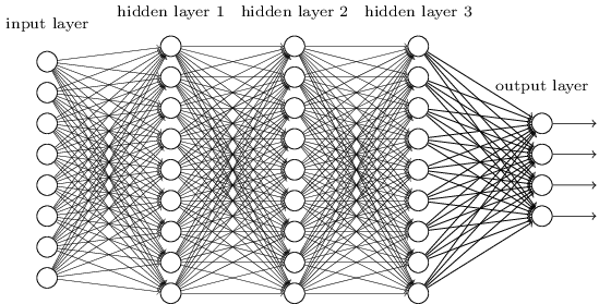
Image Recognition Bias and Symmetry

• Neural Network for image recognition
• This is a bicycle

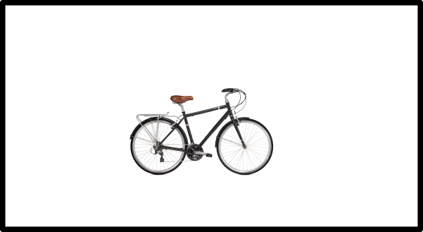
Image Recognition Bias and Symmetry

• Neural Network for image recognition
• If we shift it it is still a bicycle

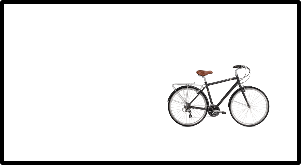
Image Recognition Bias and Symmetry

• Neural Network for image recognition
• If we shift it it is still a bicycle

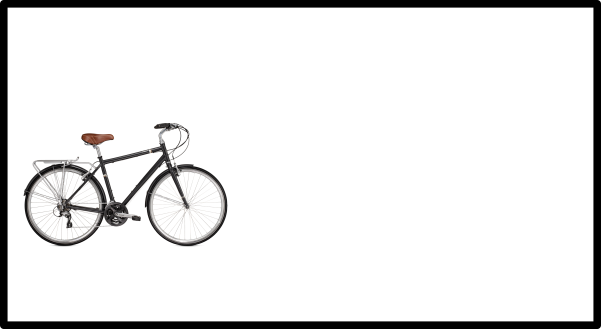
Image Recognition Bias and Symmetry

• Neural Network for image recognition
• If we shift it it is still a bicycle

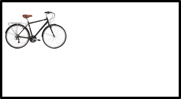
Image Recognition Bias and Symmetry

• Neural Network for image recognition
• If we shift it it is still a bicycle

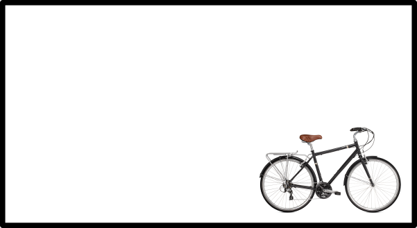
Image Recognition Bias and Symmetry

• Neural Network for image recognition
• If we shift it it is still a bicycle

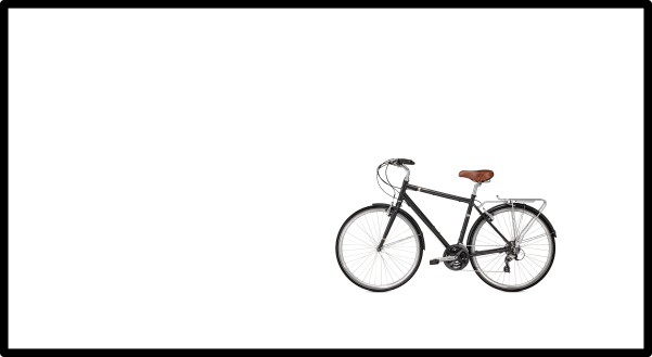
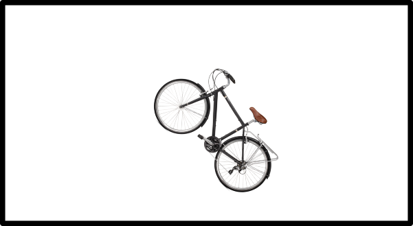
Image Recognition Bias and Symmetry

• Neural Network for image recognition
• We can even rotate it

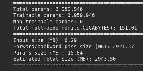
Accuracy of Fully Connected Networks

• Fully Connected Networks are not suited to image recognition

• Small well designed neural networks exceed 90% on CIFAR10
• Best networks exceed 99%

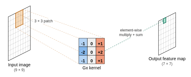
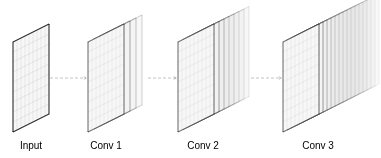
Convolution

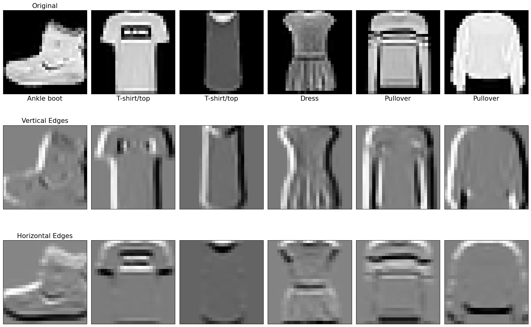
• 1960s Q: How do we detect edges in images?
• 1960s A: Create an “archetype” image of an edge, and calculate the correlation of it with each part of the original image

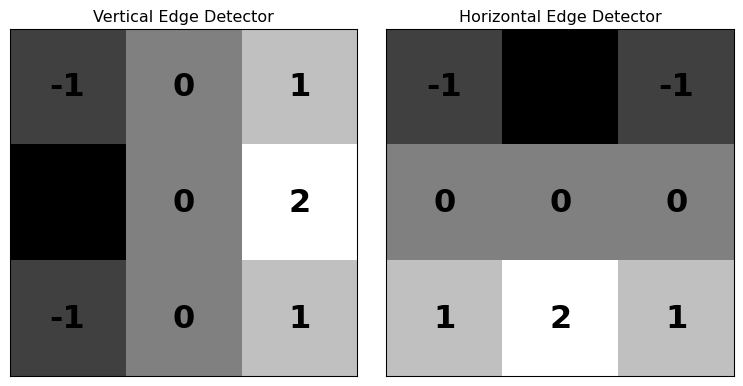
Applying the Convolution

• The convolution ‘kernel’ is like a pattern that is applied all over the target image

Convolution in Practice

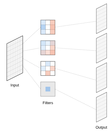
Convolutional Neural Networks

• CNN Architecture:
  • Layers are small, learned filters
  • Feature map per layer

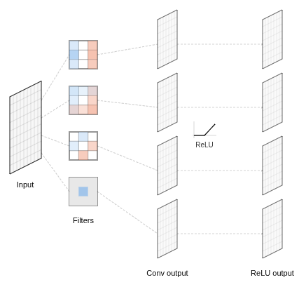
Convolutional Neural Networks

• CNN Architecture:
  • Layers are small, learned filters
  • Feature map per layer
  • Apply ReLU to feature maps

Convolutional Neural Networks

• CNN Architecture:
  • Layers are small, learned filters
  • Feature map per layer
  • Apply ReLU to feature maps
  • Stack Conv layers

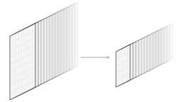
Pooling

• Convolutional layers dramatically increase the size of outputs
• Max pooling layers reduce the spatial size
• Look at 2x2 or 3x3 grid and pick maximum value

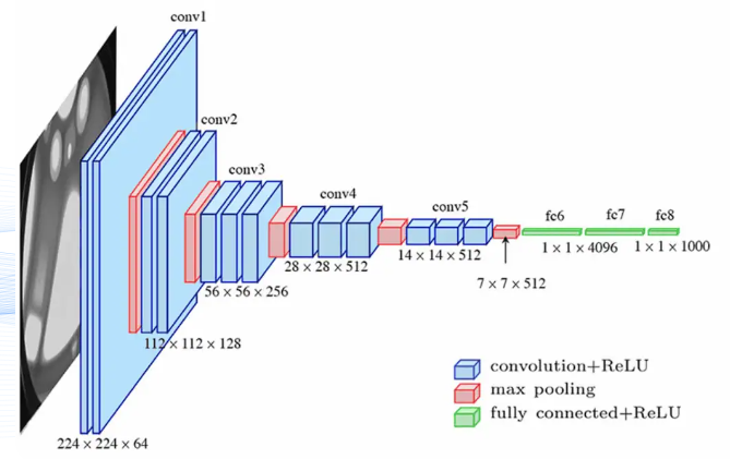
Full Architecture

• CNNs mix 1-3 Conv layers between max pooling layers
• Have some fully connected layers at the end for classification

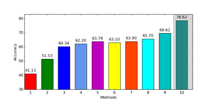
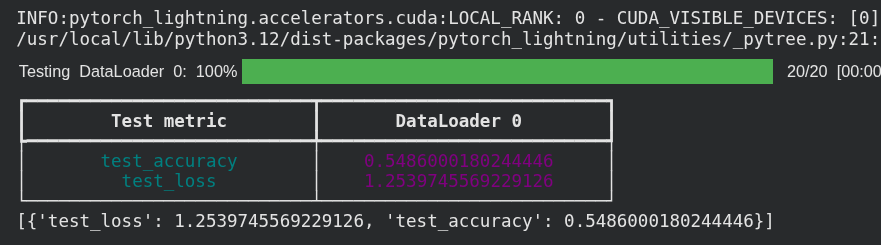
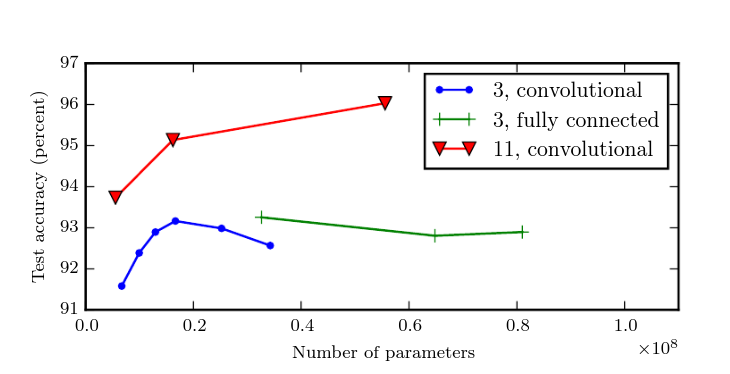
CNNs Outperform Fully Connected for Images

Fully Connected:

Fully Connected:

CNNs Outperform Fully Connected for Images

Fully Connected:

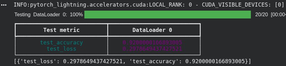
Fully Connected:

More Inductive Biases

• Translation and Rotation
  • Convolution effectively reuses weights to handle translations
• Slight change in colors, lightness/darkness
• Image being partially obscured

Data Augmentation

• Instead of modifying models, we modify training set with transformations!

transform_train = transforms.Compose([
    transforms.RandomHorizontalFlip(),
    transforms.RandomCrop(32, padding=4),
    transforms.ColorJitter(brightness=0.2, contrast=0.2, saturation=0.2),
    transforms.RandomRotation(5),
    transforms.ToTensor(),
    transforms.Normalize((0.4914, 0.4822, 0.4465),
                         (0.2470, 0.2435, 0.2616)),
    transforms.RandomErasing(p=0.5, scale=(0.02, 0.2))
])

Data Augmentation

• Instead of modifying models, we modify training set with transformations!
• Data augmentation is one of the most powerful “tricks” out there

Regularization: Dropout

• To prevent memorization, randomly zero out a fraction of neuron weights during training:

    self.output = nn.Sequential(
        nn.Dropout(0.5),
        nn.Linear(2*2*512, 512),
        nn.ReLU(),
        nn.Linear(512, 100)
    )

Regularization: Early Stopping

• Overfitting: Training loss decreases, validation loss is constant
• Solution: Stop training if validation loss has stopped improving

early_stopper = EarlyStopping(
    monitor='valid_loss',
    patience=20,
    mode='min'
)

cifar_trainer = Trainer(
    max_epochs=300,
    callbacks=[early_stopper, ...]
)

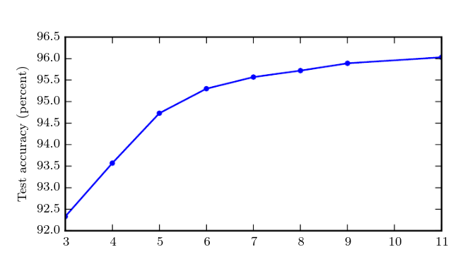
Deep Learning

• Over time, networks have become deeper
• Empirically, they lead to higher accuracy

Goodfellow et al

Deep Learning

• Over time, networks have become deeper
• Empirically, they lead to higher accuracy

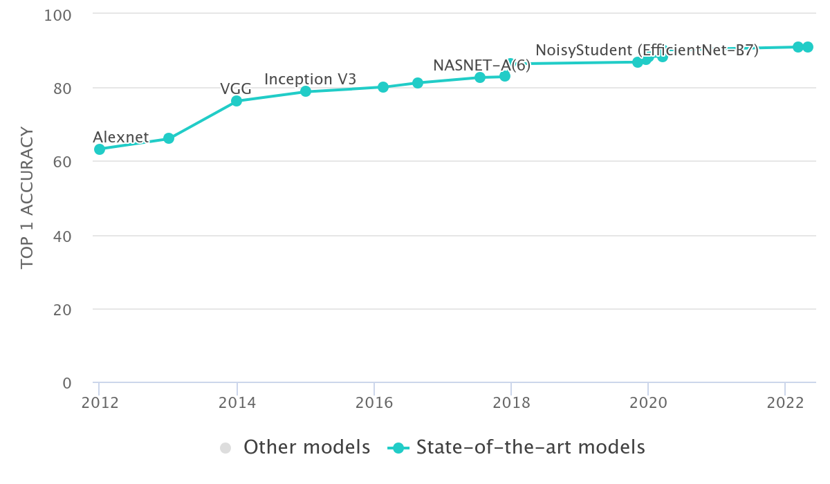
ImageNet Challenge

Different than more neurons

• Scaling up neurons often doesn’t help in shallow nets

Goodfellow

Vashing Gradients

• Landscape of deep network varies by layer:

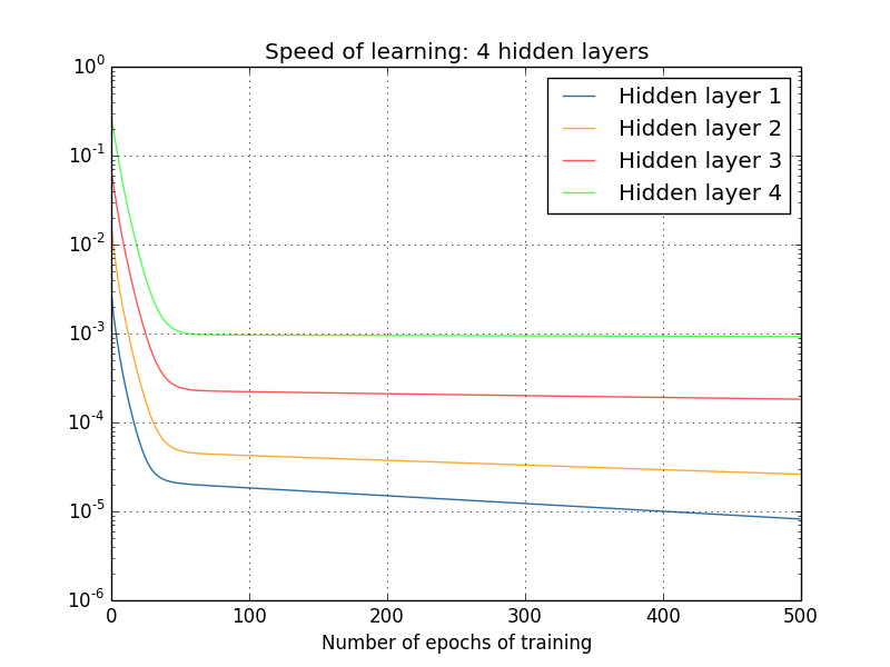
Nielson

Why Vanishing Gradients?

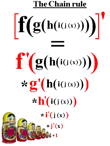
• Consider a deep network with one neuron per layer:
• If activation function is \(\phi\) can write it as: \[ f(x_1) = \phi \circ (w_n x + b_n) \circ \phi \circ (w_{n-1}x + b_{n-1}) \circ \\ \phi\circ \cdots\circ \phi \circ(w_1 x +b_1) (x_1) \]

Taking Derivatives

• The close to the output, the fewer “terms” in the derivative:

wikpedia

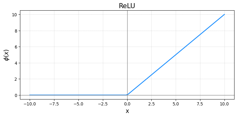
Solution: Activations

• Rectified Linear Unit (ReLU)

\[ \phi(x) = \cases{0& \text{if} \quad x\leq 0 \\ x& \text{if} \quad x>0} \]

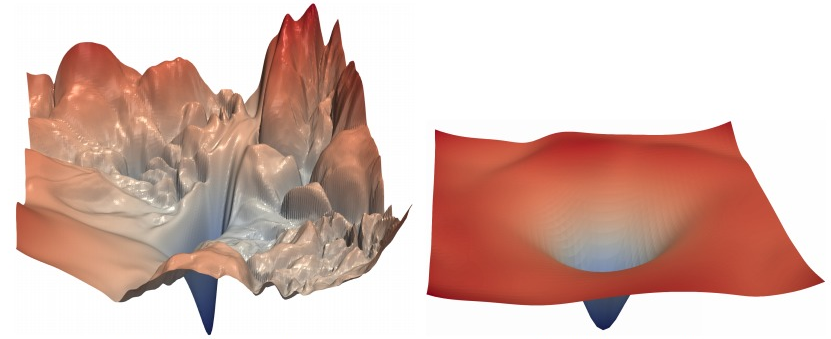
Spiky Loss Landscape

• Ideally, as you move in the direction of the gradient the loss smoothly decreases

Batch Norm

• Idea: Rescale the outputs of previous layer so that roughly 50% of neurons are active in subsequent layer
• At each batch, and each forward step, rescale data so that mean = 0 and variance is 1
• Learn an additional scaling parameter per layer
• For evaluation, using running tally of activations at each layer for normalization

Batch Norm is a Type of Layer

    self.conv1 = nn.Conv2d(in_channels, out_channels, kernel_size=3, padding='same')
    self.bn1 = nn.BatchNorm2d(out_channels)
    self.conv2 = nn.Conv2d(out_channels, out_channels, kernel_size=3, padding='same')
    self.bn2 = nn.BatchNorm2d(out_channels)
    self.conv3 = nn.Conv2d(out_channels, out_channels, kernel_size=3, padding='same')
    self.bn3 = nn.BatchNorm2d(out_channels)

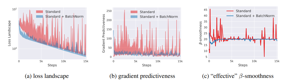
Batch Norm Enables Training Deep Networks

• Batch Norm makes the loss landscape much smoother

Thanks