DATA 622 Meetup 2: The Bias-Variance Tradeoff
2026-02-03
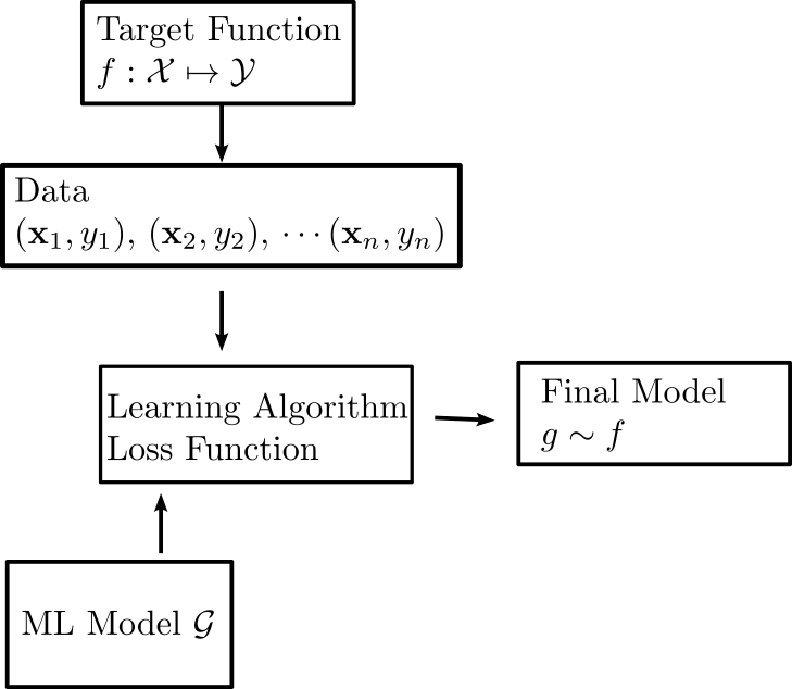
Recap: The Learning Problem
![]()
Goals
- Model Fit versus Generalization
- Bias-Variance Tradeoff
Weekly Tasks
- Lab 1 due Sunday at midnight
- Reading: ISLP 2.2-2.4
- Coding Vignette: Chapter 2 of HOML in
sklearn
- Keep posting ideas and finding team-mates in Slack
Assessing Model Accuracy
- In regression, measures like mean square error: \[
\mathrm{MSE} = \frac{1}{n}\sum_{i=1}^n (y_i - g(\mathbf{x}_i)^2)
\]
- or \(R^2:\) \[
R^2 = 1 - \frac{\mathrm{MSE}}{\mathrm{var(y)}}
\] Are used to assess model accuracy
Question:
Suppose we have trained a model which has high accuracy on the training data. Are we done?
But what we really care about is whether we can extrapolate assessed accuracy to unseen examples
Generalization
Generalization is defined as the ability of a model to maintain its accuracy on observations outside of its training
- When a model has high in-sample accuracy, it is not guaranteed that it performs well out of sample
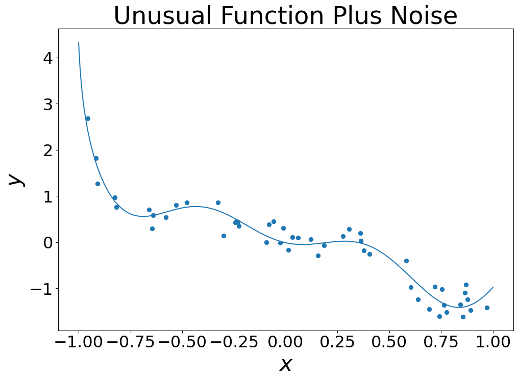
Overfitting
- Overfitting is a phenomenon that causes bad generalization
- Consider the following dataset:
![]()
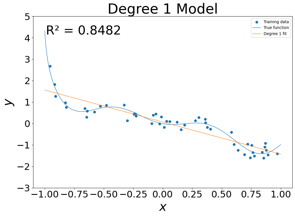
Models of Increasing Complexity
- Linear Model: \(g(x) = g_0 + g_1 x\)
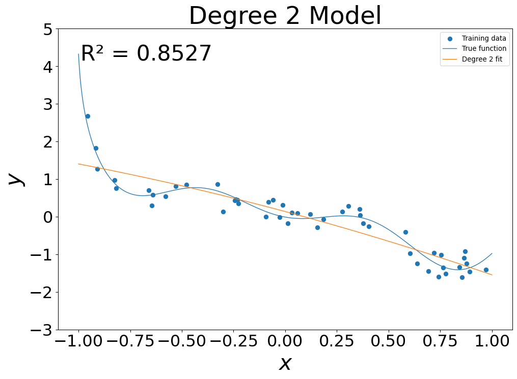
Models of Increasing Complexity
- Quadratic Model: \(g(x) = g_0 + g_1 x + g_2 x^2\)
Models of Increasing Complexity
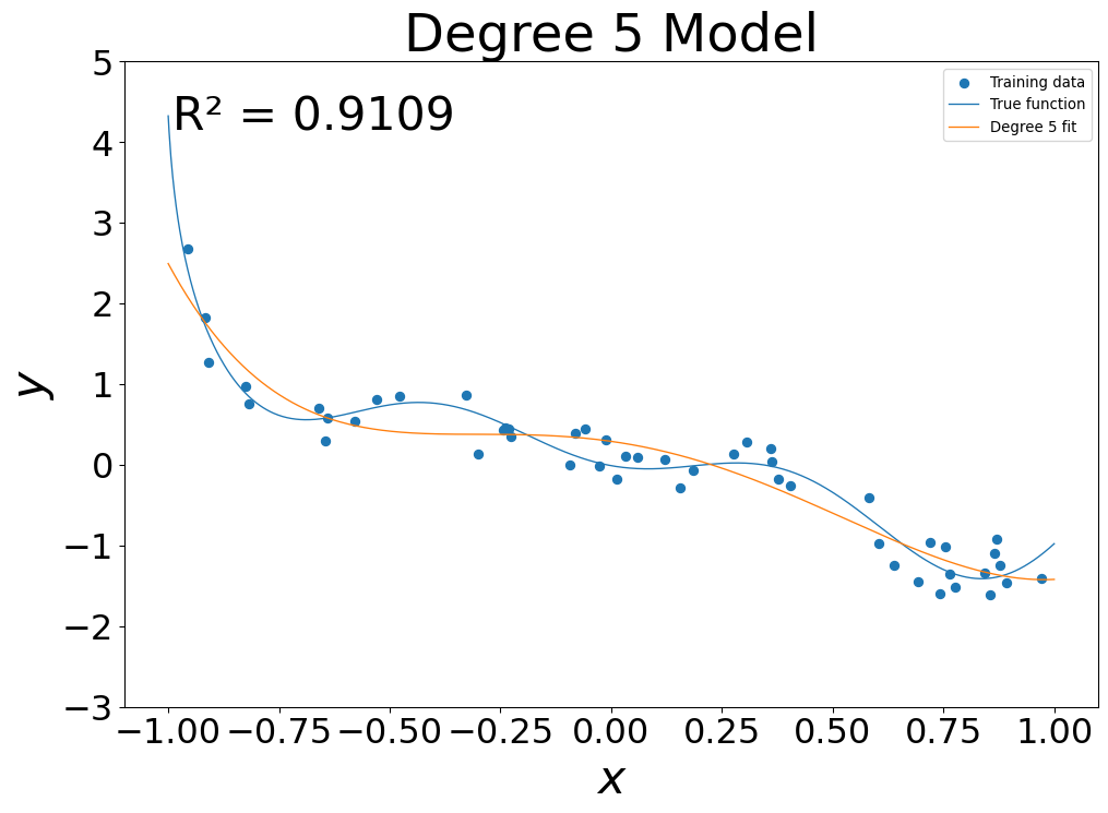
- 5th Degree fit: \(g(x) = \sum_{i=0}^5 g_i x^i\)
Models of Increasing Complexity
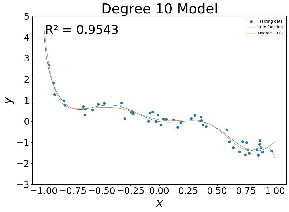
- 10th Degree fit: \(g(x) = \sum_{i=0}^{10} g_i x^i\)
Models of Increasing Complexity
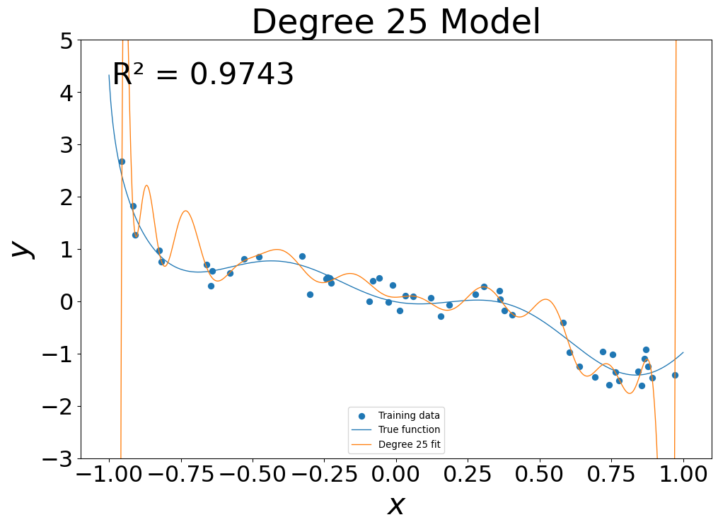
- 25th Degree fit: \(g(x) = \sum_{i=0}^{25} g_i x^i\)
Models of Increasing Complexity
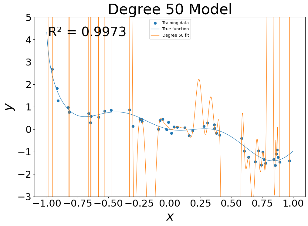
- 50th Degree fit: \(g(x) = \sum_{i=0}^{50} g_i x^i\)
Overfitting
- At low flexibility, in sample error was high
- At mid flexibility, in sample error dropped, pattern approximated
- At high flexibility, in sample error was zero
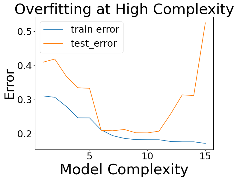
Training versus Testing Error
- Generalization Gap at high complexity
Irreducible Error
- Target function \(f(\mathbf{x})\) encodes all the information about \(y\) contained in the variables \(\mathbf{x}\)
\[
y = f(\mathbf{x}) + \epsilon
\]
- \(\epsilon\) is called the irreducible error
- It accounts for other variables that are not measured and randomness
- We have \(E(\epsilon) = 0\)
Reducible Error
- When fitting a model \(g\) to the data, there are two sources of error: \[
E((g-y)^2) = E((g-f)^2) - \mathrm{var}(\epsilon)
\]
- The \(E((g-f)^2)\) term is the reducible error
- Total error is a sum of reducible and irreducible errors
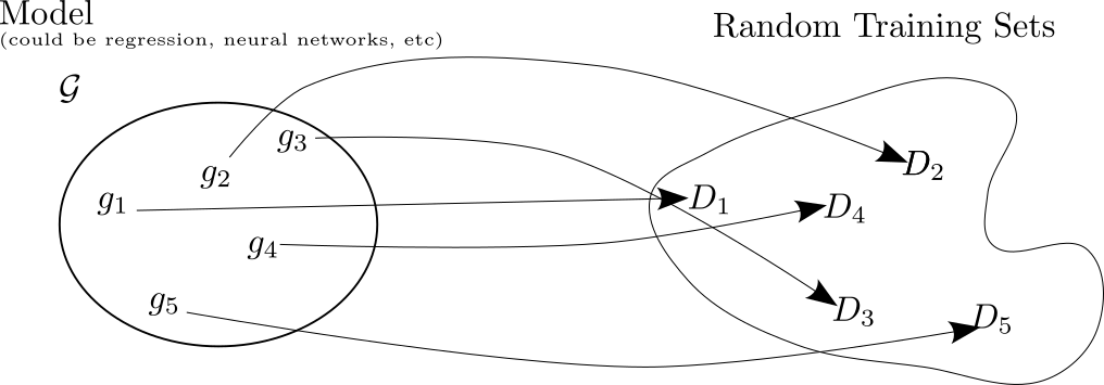
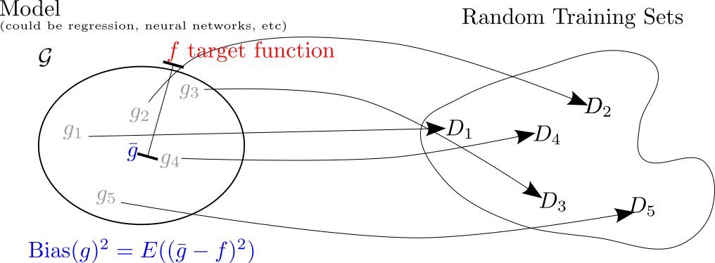
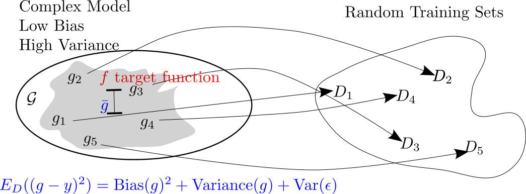
Why do complex models overfit?
- Hypothetical scenario: study the performance of a model on a repeated learning task
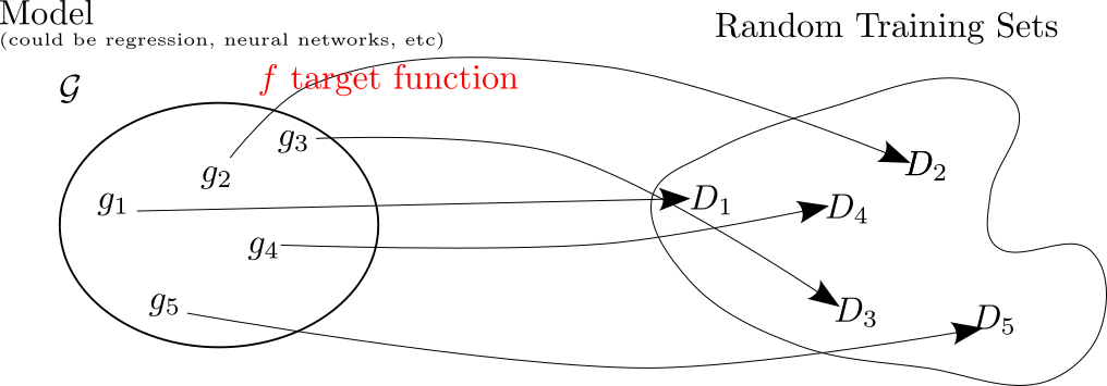
Why do complex models overfit?
- Each fit will be compared to the target function \(f\)
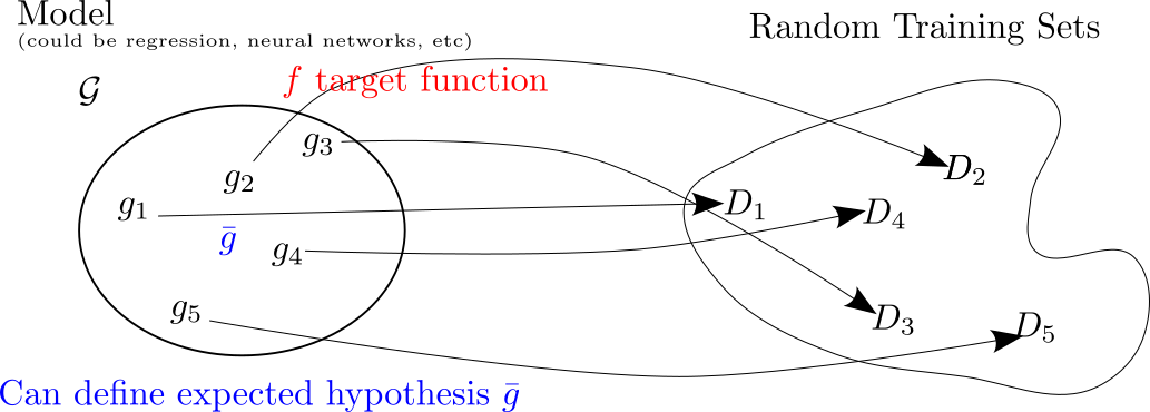
Bias Variance Tradeoff
- Can look at the “average” fit model
Why do complex models overfit?
- Bias is the distance from average fit to target
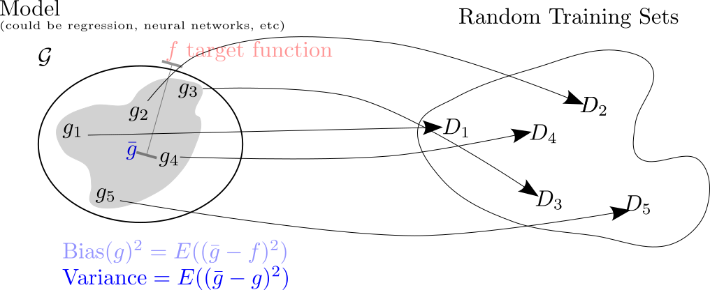
Why do complex models overfit?
- Variance is how much individual fits vary from average
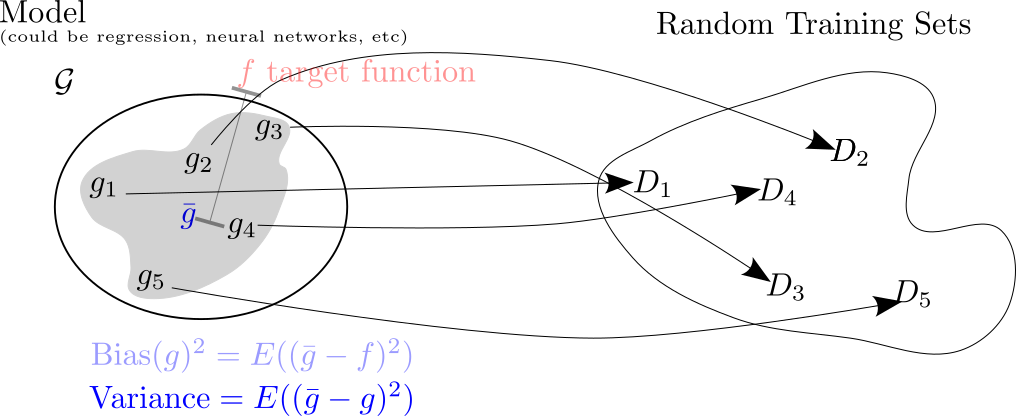
Bias-Variance Tradeoff
- Expected out of sample error is sum of squared bias, variance, and irreducible error
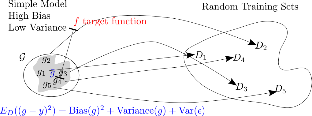
Bias-Variance Tradeoff
- Bias and variance trade-off
Bias-Variance Tradeoff
- Bias and Variance Tradeoff
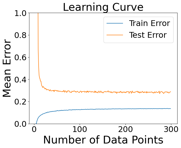
Learning Curves
- Simple versus complex models as amount of data increases
![]()
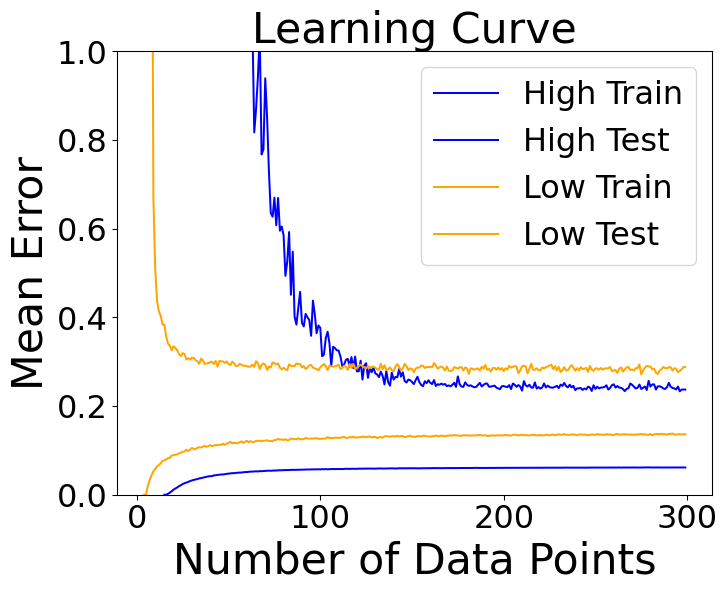
Learning Curves
- Simple versus complex models as amount of data increases
![]()
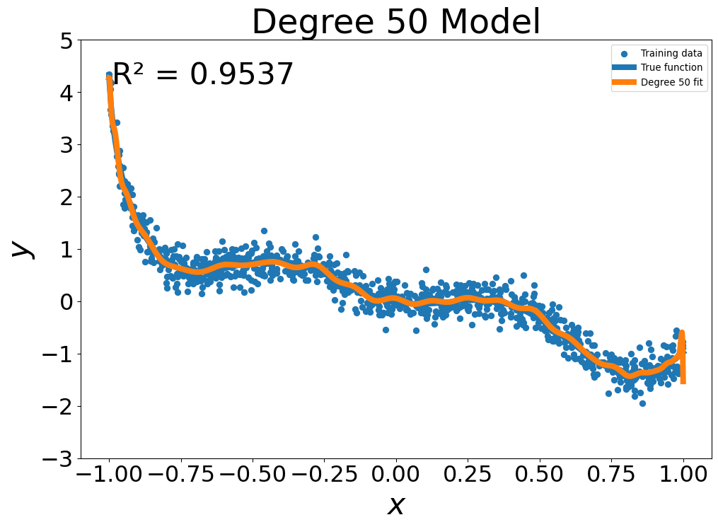
What Complexity to Pick?
Model complexity dictated by your data more so than the complexity of the phenomenon!
What Complexity to Pick?
Model complexity dictated by your data more so than the complexity of the phenomenon!
![]()
Classification Accuracy
- Switch gears to classification
- Now \(y\) is a class label
- predictors \(\mathbf{x}\) can still be continuous or discrete
Classification Accuracy
\[
\mathrm{Error} = \frac{1}{n}\sum_{i=1}^n I(g(\mathbf{x}_i)\neq y_i)
\]
- Here \(I=1\) if \(g(\mathbf{x_i}\neq y_i)\) and \(I=0\) if \(g(\mathbf{x}_i=y_i)\)
- This counts the number of times the prediction is the wrong class
Bayes Classifier
- Conditional probability of \(y\) given \(\mathbf{x}\): \[
P(y|\mathbf{x})
\]
- This is probability of class given characteristics
- Probability of default given balance, income
- Probability of hall of fame career given college stats
- Probability of disease given medical tests
Bayes Classifier
- Best prediction is to pick class with highest chance: \[
y_{\mathrm{Bayes}}(\mathbf{x}) = \mathrm{argmax}_{y} P(y|\mathbf{x})
\]
- Called Bayes Classifier or Bayes Decision Rule
Applying Bayes Decision Rule
- We don’t generally know the probabilities
- Classification models often approximate them
- Often the decision rule is basically an extension of Bayes Decision assuming good probabilities
kNN Model
- Very simple non-parametric classification model is called k-nearest-neighbors \[
g(\mathbf{x})_{kNN} = \mathrm{argmax}_{y}\sum_{\mathbf{x}_i \in N_k(\mathbf{x})} I(y\neq y_i)
\]
- Look at the \(k\) nearest points to \(\mathbf{x}\)
- Pick the \(y\) occuring most often
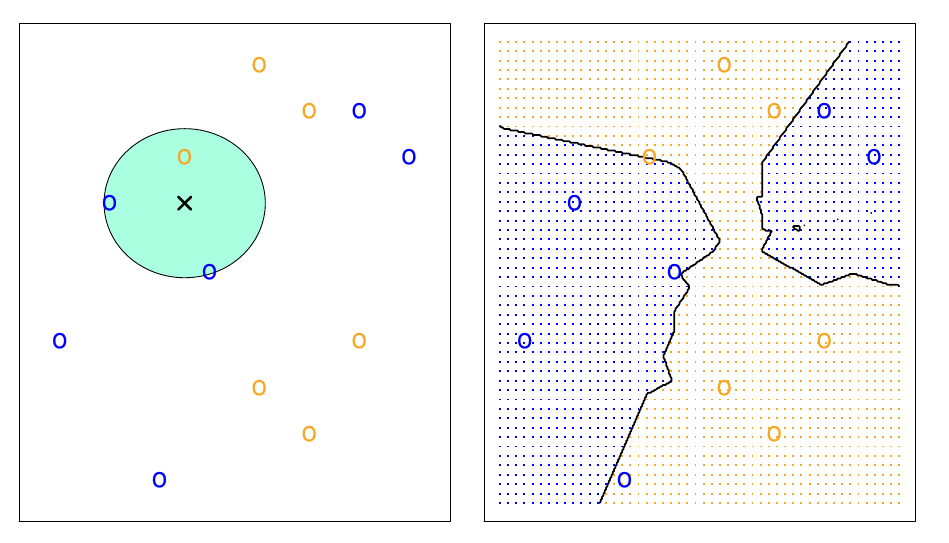
kNN Model
- Here is an example for \(k=3\).
kNN Question
- What do you think happens when \(k\) is very small?
- What about when \(k\) is very big?
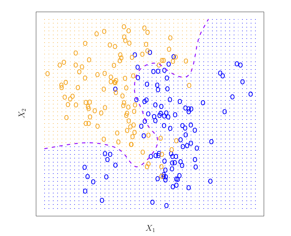
kNN Model
- Classification problem with two classes
- Boundary is the border between 50% probability of blue
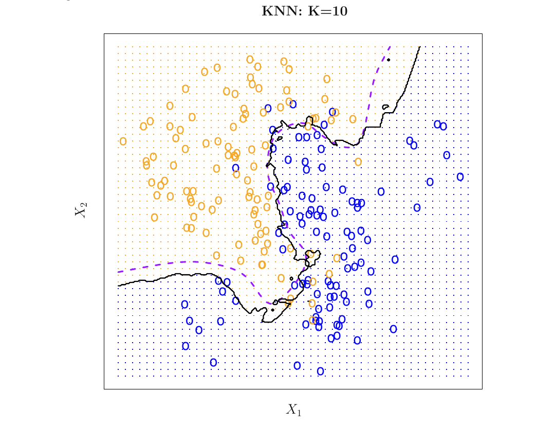
kNN Model
- Decision boundary for \(k=10\)
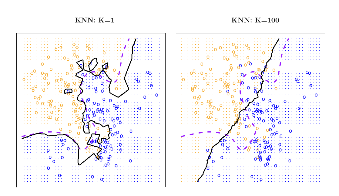
kNN Model Over and Under fitting
- \(k=1\) corresponds to overfitting
- \(k=100\) corresponds to underfitting
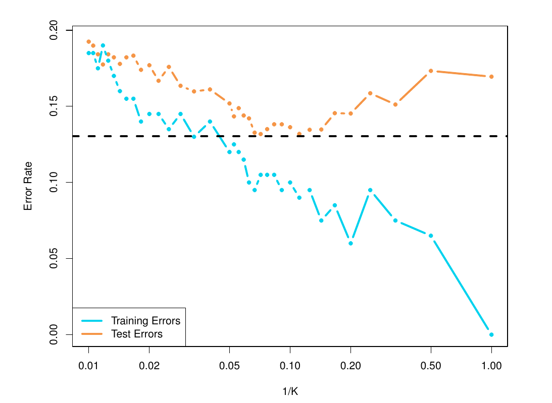
kNN Model Generalization Error
- \(1/k\) corresponds to model complexity
- Optimal out of sample accuracy at intermediate \(k\)