| Location | Loc | Population | Marriage | Divorce | WaffleHouses | South | |
|---|---|---|---|---|---|---|---|
| 0 | Alabama | AL | 4.78 | 20.2 | 12.7 | 128 | 1 |
| 1 | Alaska | AK | 0.71 | 26.0 | 12.5 | 0 | 0 |
| 2 | Arizona | AZ | 6.33 | 20.3 | 10.8 | 18 | 0 |
| 3 | Arkansas | AR | 2.92 | 26.4 | 13.5 | 41 | 1 |
| 4 | California | CA | 37.25 | 19.1 | 8.0 | 0 | 0 |
DATA 622 Meetup 3: The Linear Model
2026-02-09
nyhackr meetup Feb 17!

Why Cover this Again?
- Probably most common production ML model

Question
- What do you think are the advantages of linear regression?
Linear Models are Interpretable
- Coefficients may tell you causal effects
- Perfect for building intuition during EDA
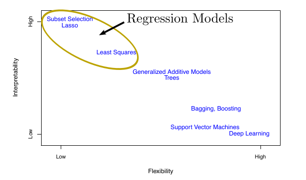
ISLP
Linear Regression Basics
- Features \(\mathbf{x} \in \mathcal{X}\):
- Combination of real numbers and categorical variables
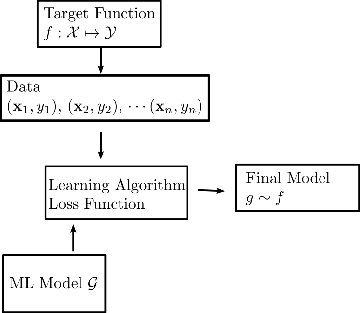
Linear Regression Basics
- Input space \(y \in \mathcal{Y}\) is just real numbers
Linear Regression Basics
- Hypotheses/Models \(g\in\mathcal{G}\) are linear functions \[ g(\mathbf{x}) = w_1x_1+\cdots w_nx_n \\ = \mathbf{w}^T\mathbf{x} \]
Linear Regression Basics
- Simplest Learning Algorithm: Minimize Loss Function \[ \mathrm{min}_{\mathbf{w}} \sum_{i=1}^n (\mathbf{w}^T\mathbf{x_i}-y_i)^2 \]
Linear Regression Basics
- Maximum likelihood with Gaussian errors: \[ L(\mathbf{w}) = \prod_{i=1}^n \exp^{-\frac{(\mathbf{w}^T\mathbf{x}_i - y_i)^2}{2\sigma^2}} \]
Linear Regression Basics
- Maximum Likelihood with Gaussian \[ L(\mathbf{w}) = \prod_{i=1}^n \exp^{-\frac{(\mathbf{w}^T\mathbf{x}_i - y_i)^2}{2\sigma^2}} \]
- Question: Do you know why?
Linear Regression Basics
- Exact Formula:
\[ \mathbf{w} = (X^TX)^{-1}X^T\mathbf{y} \]
- \(X\) is called the design matrix
- Contains the data
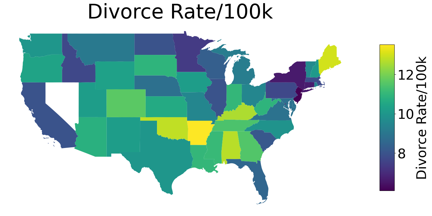
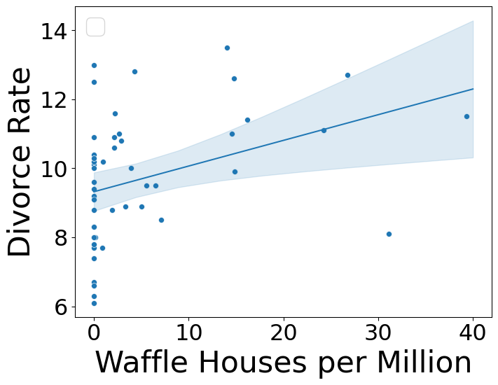
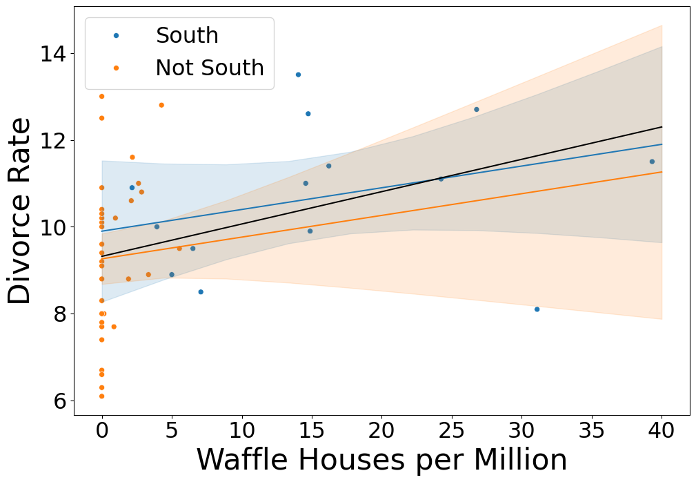
Can Waffle Houses Predict Divorce Rate?

Waffle Map

Divorce Rate Map
Confounding
Types of Confounds: Fork
- Omitted variable impacts both dependent and independent variable.
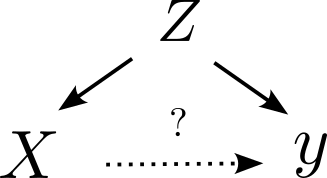
Can you tell me an example of this?
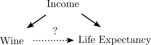
Types of Confounds: Fork
- Omitted variable impacts both dependent and independent variable.

Types of Confounds: Fork
- Omitted variable impacts both dependent and independent variable.

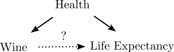
Types of Confounds: Fork
- Omitted variable impacts both dependent and independent variable.
Types of Confounds: Fork
- Omitted variable impacts both dependent and independent variable.
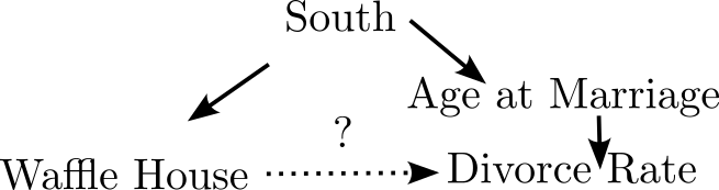
Waffle Fork
- South causes waffle house and divorce rates

Waffle Fork
- Mediated by earlier marriage age
Controlling for South
- Regression coefficient drops
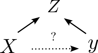
Collider Bias
Collider Bias describes a situation when the independent and dependent variable both influence a third variable which you have used in your analysis
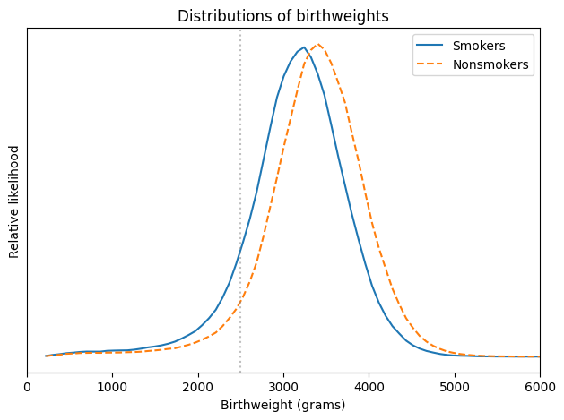
Low Birthweight paradox

- Mortality rate for low birthweight babies 25x normal weight babies
Should expectant mothers smoke?
Hint: Smokers were about twice as likely to have babies lighter than 2500 grams, which is considered “low birthweight”.
Birthweight is a Collider
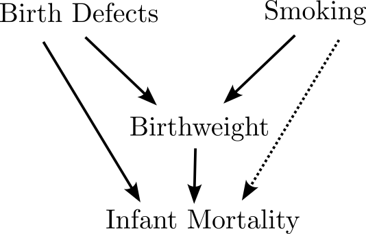
Collider Bias
- Unlike other confounders, you must not include colliders in your regression if you care about inference!
Simpson’s/Berkson’s Paradox
- This appears all over the place:
- For students already accepted to college, SAT scores don’t predict success
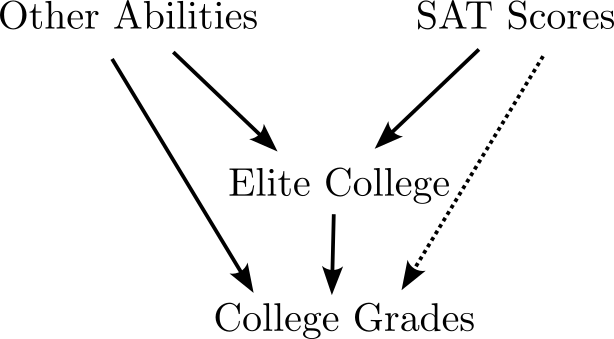
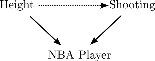
Simpson’s/Berkson’s Paradox
- This appears all over the place:
- Shorter NBA players are better at shooting than taller ones
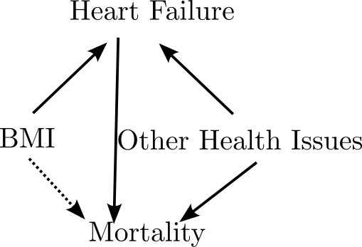
Simpson’s/Berkson’s Paradox
- This appears all over the place:
- BMI is associated with survival for heart disease patients
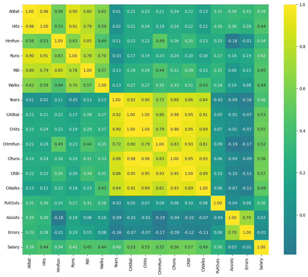
Collinear Predictors
Thanks!
![]()