| default | student | balance | income | |
|---|---|---|---|---|
| 0 | No | No | 729.526495 | 44361.625074 |
| 1 | No | Yes | 817.180407 | 12106.134700 |
| 2 | No | No | 1073.549164 | 31767.138947 |
| 3 | No | No | 529.250605 | 35704.493935 |
| 4 | No | No | 785.655883 | 38463.495879 |
DATA 622 Meetup 4: Classification
George I. Hagstrom
2026-02-16
Week Summary
- Essential to contact others about projects this week
- Proposal Due in 2 Weeks.
- Each team reach out to schedule 5-10 minute meeting during March 1 week
- HW 3 on Classification due in 2 weeks
- Coding vignette on classification/LR
HW 3 Summary:
- Always look at your figures very carefully.
- Misconception: Noise in data does not help regularize
- Later we will learn that noise in the algorithm can
- Python arrays indexed starting from 0
nyhackr meetup Tomorrow!

Weather Example
- Meteorologist forecasts the weather
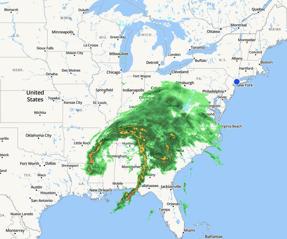
Weather Example
- Here is an example of a potential forecast:
| Day | 1 | 2 | 3 | 4 | 5 | 6 | 7 | 8 | 9 | 10 |
|---|---|---|---|---|---|---|---|---|---|---|
| Prediction | 🌧️ | 🌧️ | 🌧️ | 🌧️ | 🌧️ | 🌧️ | 🌧️ | 🌧️ | 🌧️ | 🌧️ |
| Observed | 🌧️ | 🌧️ | 🌧️ | ☀️ | ☀️ | ☀️ | ☀️ | ☀️ | ☀️ | ☀️ |
- How would you evaluate this?
Weather Example
- Which of these two forecasts do you think is better:
| Day | 1 | 2 | 3 | 4 | 5 | 6 | 7 | 8 | 9 | 10 |
|---|---|---|---|---|---|---|---|---|---|---|
| Prediction | 🌧️ | 🌧️ | 🌧️ | 🌧️ | 🌧️ | 🌧️ | 🌧️ | 🌧️ | 🌧️ | 🌧️ |
| Observed | 🌧️ | 🌧️ | 🌧️ | ☀️ | ☀️ | ☀️ | ☀️ | ☀️ | ☀️ | ☀️ |
| Day | 1 | 2 | 3 | 4 | 5 | 6 | 7 | 8 | 9 | 10 |
|---|---|---|---|---|---|---|---|---|---|---|
| Prediction | ☀️ | ☀️ | ☀️ | ☀️ | ☀️ | ☀️ | ☀️ | ☀️ | ☀️ | ☀️ |
| Observed | 🌧️ | 🌧️ | 🌧️ | ☀️ | ☀️ | ☀️ | ☀️ | ☀️ | ☀️ | ☀️ |
Which forecast is better?
It depends on the consequences of your decisions!
- Rain: Take the subway, bring umbrella
- Sun: Bike to work, no umbrella
- Cost of getting soaked on rainy day is probably higher than inconvenience of not biking or carrying an umbrella
Probability as Nuance
- What if the forecasts were like this instead:
| Day | 1 | 2 | 3 | 4 | 5 | 6 | 7 | 8 | 9 | 10 |
|---|---|---|---|---|---|---|---|---|---|---|
| Prediction | 0.8 | 0.8 | 0.8 | 0.6 | 0.6 | 0.6 | 0.6 | 0.6 | 0.6 | 0.6 |
| Observed | 🌧️ | 🌧️ | 🌧️ | ☀️ | ☀️ | ☀️ | ☀️ | ☀️ | ☀️ | ☀️ |
| Day | 1 | 2 | 3 | 4 | 5 | 6 | 7 | 8 | 9 | 10 |
|---|---|---|---|---|---|---|---|---|---|---|
| Prediction | 0 | 0 | 0 | 0 | 0 | 0 | 0 | 0 | 0 | 0 |
| Observed | 🌧️ | 🌧️ | 🌧️ | ☀️ | ☀️ | ☀️ | ☀️ | ☀️ | ☀️ | ☀️ |
Probability adds Nuance
- Consider a disease classification model
- Patient 1: \(P(\mathrm{disease}|\mathrm{labs}) = 0.001\)
- Patient 2: \(P(\mathrm{disease}|\mathrm{labs}) = 0.15\)
Both classify to “no disease”, but in patient 2 you might recommend further testing or monitoring
Calibration versus Relative Ranking
- A model with accurate probabilities is called well calibrated
- Sometimes you just need relative rankings
- Which potential customers to call?
- Which drug candidates to test?
- Where to drill test wells?
Probability Prediction Versus Classification
- Computer Science focuses on error:
\[ \frac{1}{n}\sum_{i=1}^n I(y_i \neq g(\mathbf{x}_i)) \]
- Statistics focuses on probabilities:
\[ p(y|\mathbf{x}) \]
Loss Functions for Classification
Classification often works with a threshold function: \[ g(\mathbf{x}) = 1\quad\quad \mathrm{if}\quad\quad \eta(\mathbf{x}) > 0 \\ g(\mathbf{x}) = 0\quad\quad \mathrm{if}\quad\quad \eta(\mathbf{x}) < 0 \]
Minimizing standard error function is computationally intractable!
Classification Error
- Consider this set of points:
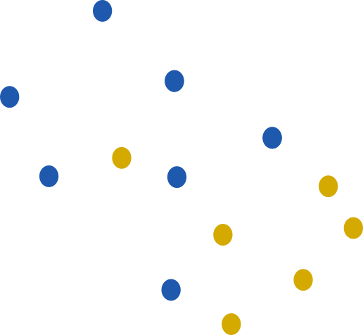
Classification Error
- Linear classifier, error is 2

Classification Error
- As we move line, error does not change

Classification Error
- Except for Sudden Jumps

Surrogate Loss
- Learning algorithms cannot use this discontinuous rule!
- Instead use surrogate functions which mimic the loss rule
- Based on threshold function
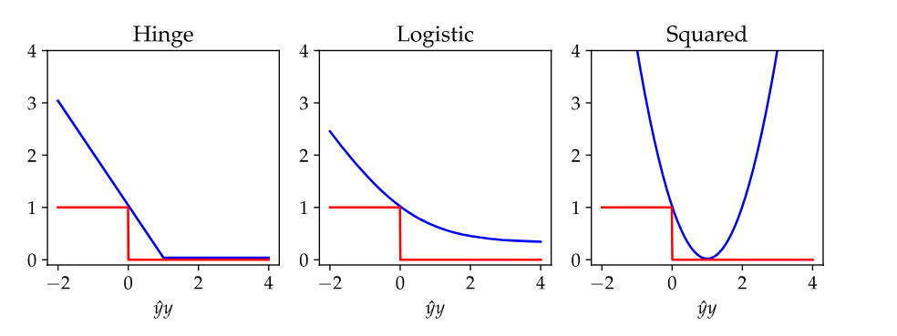
Logistic loss
- logistic function \(\sigma\): \[ \sigma(\eta(\mathbf{x})) = \frac{1}{1+e^{-\eta(\mathbf{x})}} \]
- Here is \(\eta\) is a score that could range from \(-\infty\) to \(\infty\)
- \(\sigma\) is between 0 and 1, can interpret as a probability
Logistic Regression
- \(\eta\) is linear function of predictors: \[ \eta(\mathbf{x}) = \sum_j w_jx_j \]
- Probability that \(y=1\) is \(\sigma(\eta(\mathbf{x}))\): \[ p(y=1|\mathbf{x}) = \frac{1}{1+\exp(-\mathbf{w}\cdot\mathbf{x})} \]
Maximum Likelihood for LR
- Minimizing logistic loss is equivalent to finding maximum likelihood
- ‘log’ likelihood formula: \[ L(\mathbf{w}) = \sum_{y_i = 1} \log(p(1|\mathbf{x}_i)) + \sum_{y_i=0}\log(p(0|\mathbf{x}_i)) \]
Multinomial Logistic Regression
- What happens if there are more than one class?
- Get weight vector \(w_k\) for each predictor (except last one)
\[ p(y=k|\mathbf{x}) = \frac{\exp{\mathbf{w}_k\cdot\mathbf{x}}}{1 + \sum_{j=1}^{K-1} \exp{\mathbf{w}_j\cdot\mathbf{x}}} \]
Understanding ‘log’ loss
- Consider weather examples again, interpreted as probabilities:
| Day | 1 | 2 | 3 | 4 | 5 | 6 | 7 | 8 | 9 | 10 |
|---|---|---|---|---|---|---|---|---|---|---|
| Prediction | 0.8 | 0.8 | 0.8 | 0.6 | 0.6 | 0.6 | 0.6 | 0.6 | 0.6 | 0.6 |
| Observed | 🌧️ | 🌧️ | 🌧️ | ☀️ | ☀️ | ☀️ | ☀️ | ☀️ | ☀️ | ☀️ |
| Day | 1 | 2 | 3 | 4 | 5 | 6 | 7 | 8 | 9 | 10 |
|---|---|---|---|---|---|---|---|---|---|---|
| Prediction | 0 | 0 | 0 | 0 | 0 | 0 | 0 | 0 | 0 | 0 |
| Observed | 🌧️ | 🌧️ | 🌧️ | ☀️ | ☀️ | ☀️ | ☀️ | ☀️ | ☀️ | ☀️ |
Understanding ‘log’ loss
- Misclassification Error:
- First forecast made 7 wrong predictions
- Second forecast made 3 wrong predictions
Understanding ‘log’ loss
- ‘log’ loss
- First forecast: \(3\log(0.8) + 7\log(0.4) = -7\)
- Second forecast \(3\log(0) + 7\log(1) = -\infty\)
‘log’ loss massively penalizes overconfident wrong predictions!
If this is a problem, consider using Brier score or some other loss function
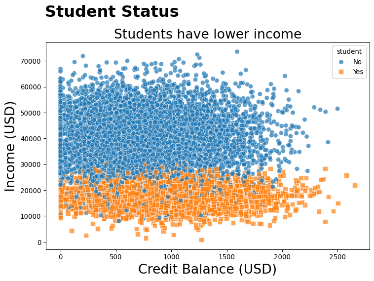
Example: Credit Data
Example: Credit Data
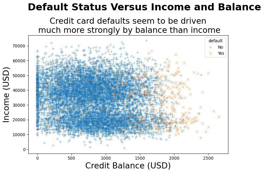
Example: Credit Data
Model Coefficients
| feature | coefficient | |
|---|---|---|
| 0 | num__balance | 2.699375 |
| 2 | cat__student_Yes | -0.518437 |
| 1 | num__income | 0.121987 |
- What do these coefficients actually mean?
logit transformation to Odds Ratios
- logistic regression predicts log-odds ratios of outcomes: \[ \log(\frac{p_{\mathrm{default}}}{1-p_{\mathrm{default}}}) = w_0 + w_1 x_1 + \cdots w_n x_n \]
- Coefficient relates feature to odds ratio
Most people do not intuitively understand log-odds ratios, nor should they be expected to be
logit transformation to Odds Ratios
- exponentiate coefficients to recover odds ratios
| feature | coefficient | odds_ratio | |
|---|---|---|---|
| 0 | num__balance | 2.699375 | 14.870429 |
| 2 | cat__student_Yes | -0.518437 | 0.595451 |
| 1 | num__income | 0.121987 | 1.129739 |
- A 1 unit change in variable leads to a change in odds equal to the ‘odds_ratio’
Marginal Effects
- Odds ratios are good, but probabilities are even more intuitive
- Doubling the odds ratio:
- 1% to 2%
- 25% to 40%
- 50% to 67%
- 90% to 95%
Marginal Effects
- To see how factors impact proability, decide where you want to make predictions
shape: (3, 3)
┌─────────┬──────────┬──────────┐
│ Term    ┆ Contrast ┆ Estimate │
│ ---     ┆ ---      ┆ ---      │
│ str     ┆ str      ┆ str      │
╞═════════╪══════════╪══════════╡
│ balance ┆ dY/dX    ┆ 0.119    │
│ income  ┆ dY/dX    ┆ 0.000202 │
│ student ┆ Yes - No ┆ -0.0103  │
└─────────┴──────────┴──────────┘
shape: (3, 3)
┌─────────┬─────────────────────┬──────────┐
│ Term    ┆ Contrast            ┆ Estimate │
│ ---     ┆ ---                 ┆ ---      │
│ str     ┆ str                 ┆ str      │
╞═════════╪═════════════════════╪══════════╡
│ balance ┆ (x+sd/2) - (x-sd/2) ┆ 0.0613   │
│ income  ┆ (x+sd/2) - (x-sd/2) ┆ 0.00269  │
│ student ┆ Yes - No            ┆ -0.0103  │
└─────────┴─────────────────────┴──────────┘
Plot the Probability Predictions
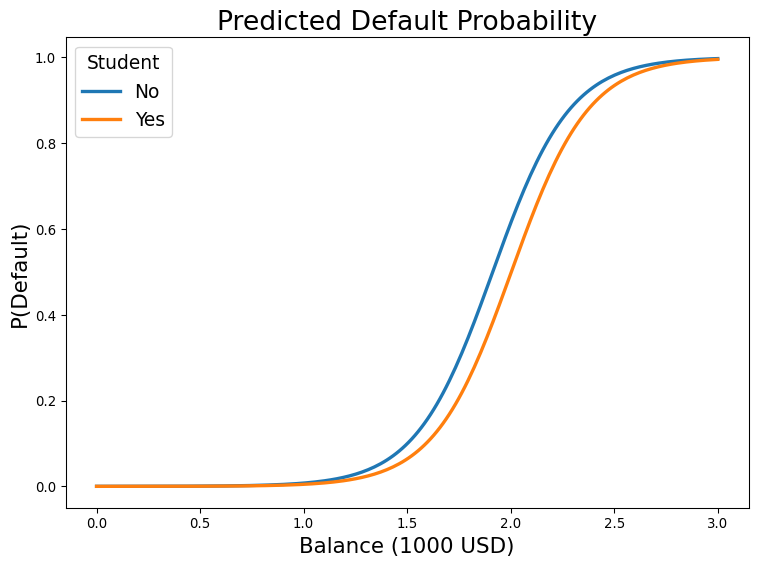
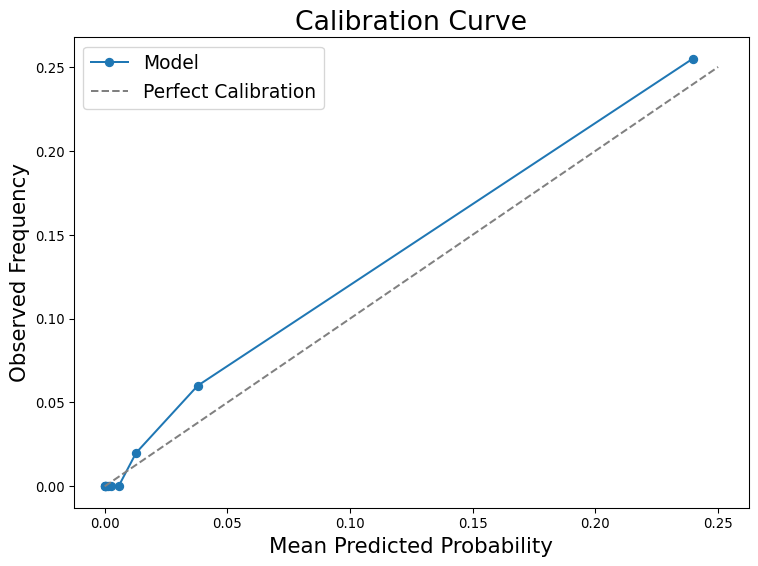
Probability Calibration
Types of errors
- Defaults are very rare, Bayes decision rule predicts no defaults!
- False Negative: predicted no default, default happened
- False Positive: predicted default, no default happened
Decision Thresholds
- Consequences of mistakes can vary:
- Predict rain wrong you accidentally carried umbrella
- Predict sun wrong, you arrived to work soaked
Solution: Bias your prediction towards the mistake that has worse consequences
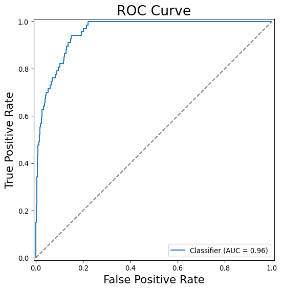
ROC Curve
Confusion Matrix
- Tabular counterpart to ROC curve
- Displays amount of different types of errors and successes
Bayes Decision Rule

              precision    recall  f1-score   support

  No Default       0.98      1.00      0.99      1933
     Default       0.75      0.27      0.40        67

    accuracy                           0.97      2000
   macro avg       0.86      0.63      0.69      2000
weighted avg       0.97      0.97      0.97      2000
- Precision: If model said it, was it true?
- Recall: If it was true, did the model say it? (TPR/TNR)
Confusion Matrix
- Tabular counterpart to ROC curve
- Displays amount of different types of errors and successes
10% threshold

              precision    recall  f1-score   support

  No Default       0.99      0.94      0.97      1933
     Default       0.30      0.72      0.43        67

    accuracy                           0.94      2000
   macro avg       0.65      0.83      0.70      2000
weighted avg       0.97      0.94      0.95      2000
- Precision: If model said it, was it true?
- Recall: If it was true, did the model say it?
Thanks
![]()
DATA 622